On the stability of intra-industry trade

著者 Hayakawa Kazunobu, Okubo Toshihiro, Ito Tadashi

権利 Copyrights 日本貿易振興機構（ジェトロ）アジア

経済研究所 / Institute of Developing

Economies, Japan External Trade Organization (IDE‑JETRO) http://www.ide.go.jp

journal or

publication title

IDE Discussion Paper

volume 542

year 2015‑10‑01

URL http://hdl.handle.net/2344/1486

IDE Discussion Papers are preliminary materials circulated to stimulate discussions and critical comments

Keywords: Two-way trade, Intra-industry trade, Stability JEL classification: F10, F14

* Tadashi ITO (corresponding author): IDE (tadashi_itoATide.go.jp) – please change AT to @., Kazunobu HAYAKAWA: IDE, Toshihiro OKUBO: Keio University, Japan

IDE DISCUSSION PAPER No. 542

On the stability of intra-industry trade

Kazunobu HAYAKAWA, Toshihiro OKUBO and Tadashi ITO*

October 2015

Abstract

This paper presents the novel finding that two-way intra-industry trade (IIT) in product–country pairs is very unstable over time by using disaggregated trade data of OECD countries. Many products frequently switch among two-way, one-way and zero trade over time. To measure the stability of two-way trade, we propose a measure that we refer to as the “IIT stability index”. Our estimation results using the proposed measure show that two-way trade involving markets of different sizes and long distance are likely to be unstable. In addition, primary products are more unstable than manufactured products.

The Institute of Developing Economies (IDE) is a semigovernmental, nonpartisan, nonprofit research institute, founded in 1958. The Institute merged with the Japan External Trade Organization (JETRO) on July 1, 1998.

The Institute conducts basic and comprehensive studies on economic and related affairs in all developing countries and regions, including Asia, the Middle East, Africa, Latin America, Oceania, and Eastern Europe.

The views expressed in this publication are those of the author(s). Publication does not imply endorsement by the Institute of Developing Economies of any of the views expressed within.

INSTITUTE OF DEVELOPING ECONOMIES (IDE), JETRO 3-2-2, WAKABA,MIHAMA-KU,CHIBA-SHI

CHIBA 261-8545, JAPAN

©2015 by Institute of Developing Economies, JETRO

No part of this publication may be reproduced without the prior permission of the IDE-JETRO.

Kazunobu Hayakawa^♠ Tadashi Ito^◆ Toshihiro Okubo^♣

October 2015

ABSTRACT

This paper presents the novel finding that two-way intra-industry trade (IIT) in product–

country pairs is very unstable over time by using disaggregated trade data of OECD countries.

Many products frequently switch among two-way, one-way and zero trade over time. To measure the stability of two-way trade, we propose a measure that we refer to as the “IIT stability index”. Our estimation results using the proposed measure show that two-way trade involving markets of different sizes and long distance are likely to be unstable. In addition, primary products are more unstable than manufactured products.

JEL F10, F14

Keywords: Two-way trade, Intra-industry trade, Stability

♠ Kazunobu HAYAKAWA: Inter-disciplinary Studies Center, Institute of Developing Economies, 3-2-2 Wakaba, Mihama-ku,

Chiba-shi, Chiba, 261-8545, Japan. E-mail: kazunobu_hayakawa@ide-gsm.org

◆Corresponding author - Tadashi ITO: Inter-disciplinary Studies Center, Institute of Developing Economies, 3-2-2 Wakaba, Mihama-ku, Chiba-shi, Chiba, 261-8545, Japan. E-mail: tadashi.ito@graduateinstitute.ch

♣Toshihiro OKUBO: Faculty of Economics, Keio University, 2-15-45 Mita Minato-ku Tokyo, Japan. E-mail:

okubo@econ.keio.ac.jp

2

1. I NTRODUCTION

Two-way trade within a sector, so-called intra-industry trade (IIT), has been one of the largest and hottest empirical research topics in the international trade literature over the last few decades. Many previous studies have proposed various methodologies to measure two-way trade and address the questions of why and how two-way trade occurs. It is a well-known fact that the current wave of globalisation has

drastically increased two-way trade. Nonetheless, it is important to note that two-way trade is not yet dominant in the real world. In other words, in addition to two-way trade, other forms of trade, such as zero trade (no trade within a sector) and one-way trade (trade between sectors), are also frequently observed. Helpman et al. (2008), using trade data on country pairs of 158 countries, show that two-way trade accounts for only 30% to 40% of country pairs, while zero trade and one-way trade account for 50%

and 10–15%, respectively, even though globalisation promotes trade liberalisation and high factor mobility. Although no previous studies have highlighted a clear relationship among the three types of trade flows, Helpman et al. (2008) provide a theoretical framework of a heterogeneous-firm trade model following Melitz (2003) to uncover how the three types of trade can co-exist. This paper adds a new finding about these three types of trade. As shown below, the three types of trade patterns are fairly unstable over time. Trade patterns frequently switch from one type to another among the three types. This dynamic aspect in trade patterns is investigated in this paper.

Our investigation yields some empirical evidence. First, trade flows among OECD countries switch between two-way, one-way and zero trade with remarkably high frequency. Two-way trade is much more unstable than expected in the previous literature. Second, the frequent switching can be explained by the GDP and geographical distance between pairs of countries. Two-way trade between large GDP countries with short distance is likely to be sustained, while this trade is more unstable when there are large

distances and gaps in GDP. Third, primary products are more unstable than machinery products.

1.1. Literature Review

Our empirical investigation follows the recent literature on IIT and can be linked with several current studies.

Related literature

Our empirical study is related to three primary strands in the literature for examining the types of trade patterns: (1) heterogeneous firm trade models, (2) stochastic trade models and (3) analysis of sequential exporting and the duration of trade.

The first strand is based on the heterogeneous firm trade model. Helpman et al. (2008) construct a

heterogeneous firm trade model and uncover the relationship among the three types of trade patterns. One of their contributions is to show the possibility of switching from two-way trade to one-way and zero

3

trade under a framework of Dixit–Stiglitz monopolistic competition by introducing firm heterogeneity as in Melitz (2003). This approach differs from the standard monopolistic competition trade models, such as those of Helpman and Krugman (1985) and Krugman (1980), which always involve two-way trade.¹² A key element of their model is the export beachhead cost, which is a sunk cost for exporting. Since firms are heterogeneous in productivity and profitability, only high productivity firms can be exporters, as they are able to use high operating profits to cover the export cost. In contrast, our focus is a stochastic aspect of trade, that is, how frequently or rapidly trade flows for a certain product in a country pair switch across two-way, one-way and zero-trade and what factors explain these switches.

The second strand examines the stochastic aspect in international trade. For example, Eaton and Kortum (2002) add the stochastic aspect to their trade model.³ They develop a probabilistic formulation by using a Ricardian type of comparative advantage model in a multi-country setting and using a continuum of goods. The model indicates the possibility that a substantial technology difference could result in a case of one-way trade and that some countries might have no exports to some foreign destinations.⁴ Much closer to our motivation is the study by Eaton et al. (2011), an extension of Melitz (2003), which provides a possible explanation to our stochastic aspect, although the main focus is neither trade patterns nor stochastic changes in trade patterns.⁵ The model involves idiosyncratic shocks to demand, export costs and productivity.⁶ In relation to our purposes in this paper, Eaton et al.’s model can be interpreted as follows: if these temporary shocks are large (e.g., negative demand shock, large positive export costs and/or negative productivity shocks), firms will not be able to export to some destinations in certain sectors, and thus zero-trade and one-way trade could temporarily arise. A possible interpretation of our

1 In the trade models with Dixit–Stiglitz-type monopolistic competition, a monopolistic competition sector always engages in two-way trade, in which goods are always produced and exported to the other country, when trade costs are finite and market sizes are not substantially different. One way to rationalize zero trade is to assume away CES function and allow choke prices, above which all demand is gone (Novy, 2013).

2 Apart from trade theory, economic geography models show the possibility of switching two-way trade to one-way trade due to full agglomeration (Fujita and Thisse, 2002; Baldwin et al., 2003). In addition, Ottaviano et al. (2002), using a linear demand function, show the possibility of one-way trade without full agglomeration. Along this line, Okubo et al. (2014) study the relationship among zero, one-way and two-way trade associated with gradual firm relocation.

3 Blum et al. (2013) highlight capital constraints and provide other evidence.

4 Finicelli et al. (2013), using the Eaton and Kortum (2002) model, provide empirical evidence on the selection mechanism and find how Ricardian comparative advantage affects trade and productivity.

5 Eaton et al. (2011) use the trade model of Eaton and Kortum (2002) combined with firm heterogeneity as in Melitz (2003) to empirically test hypotheses against French microdata.

6 Eaton et al. (2011) model export-related fixed costs, which include a fixed-cost shock specific to a product and a destination, as well as marketing cost as in Arkolakis (2010).

4

findings discussed below is that these temporary shocks may result in frequent switching among the three types of trade flows.⁷

The third strand examines sequential exporting and the duration of trade. The duration of exporting products is very short and the hazard rate sharply declines over time (Besedes and Prusa, 2006). Many exporters are likely to give up exporting after a short period due to product- or destination-related shocks, which results in temporary trade (Békés and Muraközy, 2012).⁸ A different aspect from this evidence is learning by exporting and sequential exporting. Albornoz et al. (2012), Papageorgiou and Arkolakis (2009) and Buono and Fadinger (2012) find that firms have difficulty initiating exports due to sunk costs.

However, once they start trading, firms learn about foreign markets and thus will face lower demand uncertainty in future periods. In contrast, less productive firms are more likely to stop trading as a result of experiencing demand uncertainty. Although these studies are not directly linked to ours, they can support our empirical finding that IIT at the product-destination level may be less likely to endure over time.

IIT literature

Our empirical strategy is based on the IIT literature. The measure of IIT most commonly used in the literature is the Grubel–Lloyd (GL) index (Grubel and Lloyd (1975)). In the literature, conventional IIT is classified into two types: horizontal IIT (HIIT) and vertical IIT (VIIT). HIIT is defined as IIT without a substantial per-unit export and import price gap. In contrast, VIIT is defined as IIT with a substantial per- unit export and import price gap. The HIIT and VIIT indices were first proposed by Greenaway et al.

(1995) and have subsequently been used by many authors. Using category-level UK trade data from 1988 under the five-digit Standard International Trade Classification system, Greenaway et al. (1995)

empirically investigated the determinants of HIIT and VIIT. Subsequently, Aturupane et al. (1999) and Jensen and Lüthje (2009) studied the determinants of HIIT and VIIT using trade data between the EU and Central and Eastern European transition economies from 1990 to 1995 and from 1996 to 2005,

7 The theory of export hysteresis provides the opposite hypothesis, that firms’ export statuses are highly persistent. This theory was first developed by Baldwin and Krugman (1989) and Dixit (1989). When sunk costs for exporting are substantially large, producers do not start exporting unless the present value of expected future export profit is sufficiently large. Yet, once they start exporting, exporters continue in an exporting status even when their net profits become negative. These studies indicate that large entries into exporting are not frequent and trade patterns are fairly persistent. Consistently, previous empirical studies have shown that exporting status is persistent. According to Das et al. (2007) and Roberts and Tybout (1997), sunk costs for exporting are substantially large and thus producers do not start exporting unless the present value of expected future export profit is large enough. More currently, Impullitti et al. (2013) introduce idiosyncratic firm productivity shocks to the

heterogeneous firm trade model on the time continuum. The shocks evolve over time following a Brownian motion stochastic process. They show that firms keep exporting even when there is a large drop in productivity.

8 Elliott and Tian (2010a) (2010b) evaluate sequential exporting to Asia and Europe by Argentinean firms.

5

respectively. Brülhart (2009) provided a comprehensive description of global IIT and inter-industry trade patterns using worldwide category-level trade data under the six-digit Harmonized System (HS).

The IIT indices mentioned above are all static. Closer to our interest, it is important to illustrate transitional changes in long-run trade patterns. To deal with the dynamic aspect, the notion of marginal IIT (MIIT) is proposed to measure structural change in trade patterns. An important issue in MIIT is labour market adjustment. Many researchers found a negative relationship between MIIT and adjustment pressure. For example, Brülhart and Elliott (2002), Brülhart et al. (2006) and Cabral and Silva (2006) proposed empirical tests of the smooth-adjustment hypothesis (SAH) associated with MIIT. According to the SAH, the adjustment costs associated with inter-industry trade are higher than those associated with IIT because a change in the former generally requires greater resource reallocation.⁹

While the studies on MIIT and SAH focus on changes in IIT over time, our paper focuses on the change in trade patterns, which shifts between two-way trade and the other trade patterns. Thus, our paper is essentially different from the MIIT literature.

Our paper aims to provide some empirical evidence on how and why the three types of trade flows frequently switch over time. For our purposes, “stability” in IIT means no frequent changes in the trade type and sustained IIT. On the other hand, “instability” is defined as the frequent switching among the three types of trade. This paper adds the concept of IIT stability to the literature, starting from the standard IIT methodology.

The rest of the paper is organised as follows. The next section explains the data and the Grubel–Lloyd IIT index and its decomposition. Section 3 proposes an index to measure the stability of IIT and examines the determinants of IIT stability. The final section provides concluding remarks.

2. D ATA AND G RUBEL –L LOYD IIT I NDEX

This section describes the evolution of the conventional IIT index using the GL index. We use OECD country trade data at the 6-digit HS category level for the period of 1994 to 2010. Data are from the UN COMTRADE database. The analyses use the 28 OECD countries, and the choice of the period (1994 to 2010) is based on the longest possible length of time that allows for balanced panel data in terms of the coverage in each year. A balanced panel is required for our type of analysis because the period of data coverage needs to be identical across countries to compute and compare the IIT stability index, as will be explained below.

The GL index of product category pbetween country i and j at time t is defined as

9 Early contributions on this issue were made by Hamilton and Kniest (1991), Greenaway et al. (1994), Brülhart (1994) and Azhar et al. (1998).

6

𝐺𝐺𝑖𝑖𝑖𝑖 ≡ 1 −�𝑇𝑇𝑇𝑇𝑇_{𝑖𝑖𝑖𝑖}− 𝑇𝑇𝑇𝑇𝑇_{𝑖𝑖𝑖𝑖}� 𝑇𝑇𝑇𝑇𝑇𝑖𝑖𝑖𝑖+ 𝑇𝑇𝑇𝑇𝑇𝑖𝑖𝑖𝑖 ,

where Tradeijpt refers to exports of product p from country i to country j at time t. The second term represents the index of inter-industry trade. The index of intra-industry trade is computed as one minus the index of inter-industry trade, namely, as the residual.

An aggregate index of total IIT between two countries is conventionally computed by using the share of trade values as weights (e.g., as in Jensen and Lüthje, 2009).

𝐼𝐼𝑇_𝑖𝑖𝑖 ≡ ∑_𝑖∈Ω�𝑤_{𝑖𝑖𝑖𝑖} × 𝐺𝐺_{𝑖𝑖𝑖𝑖}�, where 𝑤𝑖𝑖𝑖𝑖 ≡ _∑ ^{𝑇𝑇𝑇𝑇𝑇}_{�𝑇𝑇𝑇𝑇𝑇}^{𝑖𝑖𝑖𝑖+𝑇𝑇𝑇𝑇𝑇𝑖𝑖𝑖𝑖}

𝑖𝑖𝑖𝑖+𝑇𝑇𝑇𝑇𝑇_{𝑖𝑖𝑖𝑖}�

𝑖∈Ω .

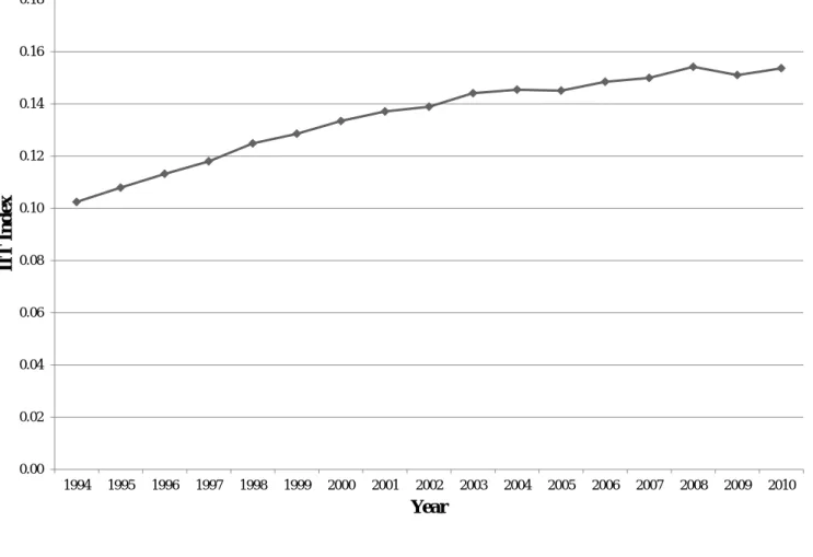
Ω indicates a set of all products. Using this, the IIT index is calculated for all the country pairs and the simple average is taken. The evolution of the IIT index is shown in Figure 1. As has been documented in the IIT literature, the IIT index has been increasing over time.

3. S TABILITY OF IIT R ELATIONSHIPS

This section proposes an IIT stability index. Our analysis reveals that IIT is rather unstable for individual country-product pairs, even though the aggregate IIT index has been steadily increasing over time, as shown by the previous literature and Figure 1 in the last section. The descriptive analysis shows that highly developed OECD countries tend to have high IIT stability indexes compared with the other OECD countries. The econometric analysis indicates that the conventional gravity variables explain the stability of IIT relationships well.

3.1. Stability of IIT: A simple counting of IIT trade years

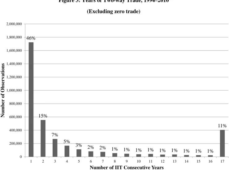
To examine the stability of the IIT of a particular product between a pair of countries, we have counted the number of years (maximum 17 years) a certain product is recorded as having two-way (IIT) trade between a pair of countries in the period from 1994 to 2010. Figure 2 shows the shares by the number of years that IIT is recorded in country–product pairs. About half of the sample (51%) have “zero” IIT, which means zero trade or one-way trade was observed consistently over all sample years. On the other hand, the other half (49%) have IIT. IIT in all sample years (17 years) accounts for only 11%, whereas IIT recorded for a few years (between 1 and 5 years) accounts for 20%. This result indicates most goods are traded intermittently, that is, moving between one-way trade and two-way trade (IIT). To focus more on one-way and two-way trade, Figure 3 shows how many years IIT can be consecutively continued: the

7

frequency of the number of years consecutively recorded as IIT.¹⁰ The length of two-way trade ranges from 1 to 17 years. This means that, for most products, IIT is difficult to maintain in consecutive years, meaning that trade is kept up for just for 1 or 2 years. In total, we can conclude that IIT is fairly unstable over time.

3.2. IIT stability index

Although this simple count of years of IIT is straightforward and useful to gain an initial grasp of the rather unstable nature of IIT relations, it does not distinguish between, for example, seven years of intermittent IIT out of the total 17 years and seven years of consecutive IIT out of the total 17 years. It is natural to consider that seven years of consecutive IIT is more stable than seven years of intermittent IIT.

Given that, in the current global economy, the structure of economies changes rapidly, it is natural that countries change their comparative advantage within short periods of time. Also, it is important to note that the average survival period of firms is far less than 17 years, which also contributes to instability and changing conditions. Thus, we propose the following IIT stability index. It is defined as:

( )

17

1

1 1

153 2

ijp k

k

Stability X k k

=

+

 

 

≡ 

∑

where X_k is the number of k-consecutive years of "wins" (IIT) in the 17 years period. We refer to the

part ¹⁷

( )

1

1

k 2

k

X k k

=

 + 

 

 

∑

2 , is the cumulative number of years. For example, the case of 17 consecutive years of IIT (the whole sample period) yields the sum from n=1 to 17, that is, ∑ 𝑛¹⁷₁ = ^17∗18₂ = 153, whereas the case of a single year of IIT gives a score of 1 and a case of two consecutive years is 1+2=3. Hence, the general case of k consecutive years is given by

∑ 𝑛^𝑘1 = ^𝑘(𝑘+1)₂ .

In words, the scoring rule of this index is to add one point when the product switches from non-IIT to IIT and then, if it continues to be recorded as IIT for the subsequent years, an incremental score is added. Any incremental score could be used, as further explained below. However, our definition adopts the simple rule of increasing the increment by one for each consecutive year of IIT.

10 For example, when IIT is observed between two countries in 1995, 1996, 2000, 2005 and 2006, the numbers of observations are one for a single IIT year and two for two consecutive years of IIT.

8

To finalise the explanation, the score of k-years of consecutive IIT is multiplied by the number of runs of k-years of consecutive IITs, X_k. For example, if IIT is recorded for the years 1995 and 1996 (two

consecutive years), the years 2000, 2001 and 2002 (three consecutive years) and for the years 2005 and 2006 (two consecutive years), the score for two consecutive years (here, a score of 3) is counted twice (1995–1996 and 2005–2006), giving X₂ =2, and the score for three consecutive years (here, a score of 6) is counted only once (for 2000–2002), namely X₃ =1, making the total score 3*2+6*1=12. To convert this score into an index that takes a value in

[ ]

( )

17

1

1 1

153 2

ijp k

k

Stability X k k

=

+

 

 

≡   

 

∑

with k=2, 2(2+1)/2 and k=3, 3(3+1)/2 normalisation X2=2 (twice two consecutive years (k=2) of IIT) X3=1 (once three consecutive years (k=3) of IIT) To ease readers’ comprehension of this counting rule, a simple numerical example is provided in the appendix A.1. Hereby, the stability index for each product pfor a pair of country i and j is computed.

To compute the aggregate IIT stability index for a pair of countries i and j, we adopt the following weight.

𝑣𝑖𝑖𝑖 ≡ ∑ 2 × min�𝑇𝑇𝑇𝑇𝑇_𝑖 𝑖𝑖𝑖𝑖, 𝑇𝑇𝑇𝑇𝑇_{𝑖𝑖𝑖𝑖}�

∑ ∑_{𝑖 𝑖∈Θ𝑖}2 × min�𝑇𝑇𝑇𝑇𝑇_{𝑖𝑖𝑖𝑖}, 𝑇𝑇𝑇𝑇𝑇_{𝑖𝑖𝑖𝑖}�

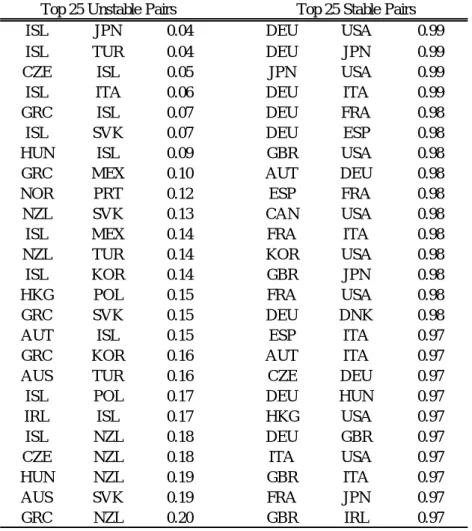
Here, Θt indicates the set of products categorised as IIT in year t. The result for the top 25 stable and unstable pairs of countries is shown in Table 1. We tried several other incremental rules (such as

additional scores of 2, 3, or 4, or geometric progression),¹¹ and obtained qualitatively equivalent results.

The country groups illustrate substantial contrast. Top ranked countries in terms of both stability and instability are composed of similar countries in each group. IIT among highly developed countries is relatively stable, while IIT among new OECD countries is relatively unstable. Stated differently, trade between large countries is likely to be stable, while trade between small and peripheral countries is unstable.

11 For example, if we adopt a rule providing an additional 2 points for each consecutive IIT year, then a three consecutive year period of IIT earns a score of 9 (=1+3+5). Or, if we adopt a geometric progression, then a possible score is 14 (=1+4+9).

9

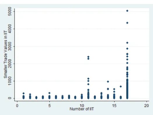
One possible concern could be that unstable IIT might be caused simply by the smaller trade values for the new and peripheral OECD countries rather than the stock of IIT goods themselves. Namely, goods with small trade values can easily change to zero trade due to relatively small shocks, whereas goods with large trade values do not shift to zero trade by the same small shocks. To check this, we have plotted the export or import value in country–product pairs, whichever was smaller, by the number of IIT years. As Figure 4 shows, although the values for highly persistent IIT with 16 or 17 consecutive years are

relatively high, there is no evidence that lower values for consecutive IIT years are correlated with lower trade value (export or import, whichever smaller). Thus, the difference between stable and unstable IIT products does not seem to have been caused simply by their trade values.

3.3. Sensitivity analysis

Now we investigate the relationship between the stability index and the IIT index. Figure 5 plots the country-pair stability index in terms of the number of IIT products. Country pairs with a small number of IIT products have a large variation for the stability index, while country pairs with a large number of IIT products converge to high stability.

It is natural that large IIT country pairs result in a higher stability index because many of their IIT

products are likely to have consecutive years of transaction. In contrast, low-IIT country pairs do not have an obvious cause. Even if one-way or zero trade are highly dominant, IIT might be stable if a small number of IIT products maintain consecutive years of transaction. Or, more importantly, another possibility is that IIT fluctuates over time with frequent switches to one-way or zero trade, which

indicates unstable and lower IIT. Another possibility is the occurrence of spot transactions. For instance, this would occur for a product that is traded once every few years. As a result, there is a single year or a few years of IIT and other years are one-way or zero trade.

Furthermore, the so-called “partial year effect” may have an impact.¹² Trade data available across many countries, as in the case of this paper, are on an annual basis for the period from January to December.

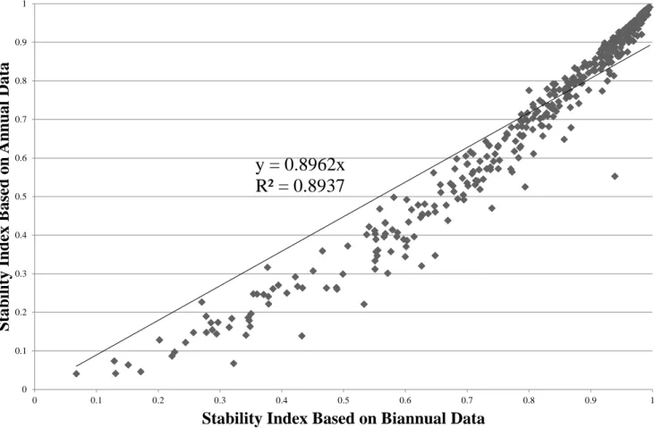
Thus, regular annual shipments in December are usually recorded in the respective year, but delays of shipments often take place. Thus, if a December shipment is delayed by one month and occurs in January, that shipment is recorded in the next calendar year. In order to check if the annual nature of the data affects our index, we also compute the stability index using 2-year trade data, which are constructed by aggregating the annual data for each 2-year period. The relationship between these two methods for constructing the stability index is depicted in Figure 6. Since the slope is almost one and R-squared is high, the nature of trade statistics in terms of time does not seem to significantly affect our index.

12 See Bernard et al. (2013) for more detail. According to them, a partial year effect is one in which “the concept is quite simple, almost trivial, yet the implications for the existing stylized facts on export levels and growth rates are profound.”

10

4. D ETERMINANTS OF IIT STABILITY

4.1. Country size and distance

To investigate what kind of attributes of country pairs affect IIT stability, this subsection runs regressions of the aggregate IIT stability index computer above on certain pair-specific variables. Specifically, we examine the roles of real GDP, GDP per capita, geographical distance (Distance), linguistic commonality (Language), border-sharing (Contiguity), and real exchange rate volatility (Volatility). Real GDP and GDP per capita (unit: US dollar) are taken from the World Development Indicators (World Bank), real exchange rate is from the International Financial Statistics (IMF) and the data source of geographical distance (unit: kilometre), language and border-sharing is CEPII. In terms of GDP, we use the product between the average GDPs during the period 1994-2010 in the two trading countries (GDP Product).

GDP is deflated by the GDP deflator. The same kind of product is computed for GDP per capita (GDP Capita Product). Following the gravity literature on exchange rate volatility (e.g., Rose, 2000), we compute volatility as the standard deviation of the first-difference of the monthly natural logarithm of bilateral real exchange rates during the period 1994–2008. The descriptive statistics for the variables are provided in the appendix A.2.

Estimation results are shown in Table 2. Column (I) reports our results in terms of ordinary least squares (OLS). GDP, GDP per capita and language are significantly positive, and distance and exchange volatility are significantly negative. Thus, IIT is likely to be stable in country pairs with large markets, high

economic development, low exchange rate volatility, geographical proximity, linguistic commonality, or border-sharing. In essence, two large countries with short geographical distance between them are more likely to stabilise trade patterns and maintain two-way trade over time. As shown in column (II), these results do not change qualitatively even if we estimate our model by employing the fractional logit model proposed by Papke and Wooldridge (1996), which may be a suitable estimation technique for a model with a unit-interval dependent variable.¹³ One noteworthy difference is that the coefficient for Contiguity turns out to be significantly positive, implying that IIT is likely to be stable in country pairs with shared borders. We note that all of these results are unchanged by using different weights in the aggregation of

13 The fractional logit model ensures that, unlike with OLS, the predicted values of the dependent variable are in the unit interval. Also, unlike the log-odds ratio model and the beta regression model, it can naturally define dependent variables for the boundary values 0 and 1. It imposes less restrictive assumptions than the Tobit model (which requires normality and homoskedasticity of the dependent variables). For more details, see Ramalho et al. (2011).

11

the IIT stability index for country pairs.¹⁴ In column (III), we also run regressions on the non-aggregated version of the IIT stability index, that is, Stabilityijp. The results are qualitatively unchanged.

Eaton et al. (2011) may provide some possible explanations for our findings. High exchange rate volatility and no linguistic commonality increase the volatility and level of export costs, leading to unstable IIT. Country pairs involving small economies have lower GDPs and lower per-capita income;

thus, demand shocks are likely to be more idiosyncratic and uncorrelated, which also leads to unstable IIT.

Furthermore, while this is not a direct interpretation from our estimation results, Eaton and Kortum (2002) imply that small countries may have a substantial comparative advantage in some specific sectors and specialise in and export the products of these comparatively advantageous sectors. As a result, small countries may be more likely to have unstable IIT.

4.2. Product variation

As shown in the last subsection, country characteristics are key determinants for the stability of IIT.

However, product aspects are also worthwhile to mention. In order to examine the product variation, we investigate the stability index aggregated by product sector, as defined in the HS classification.¹⁵

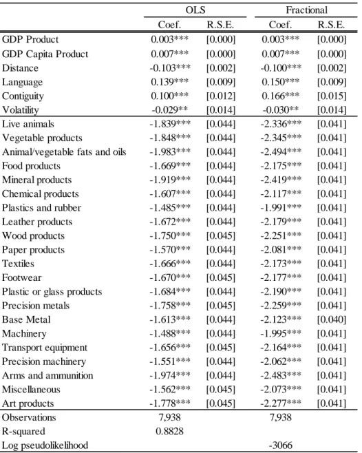
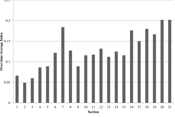
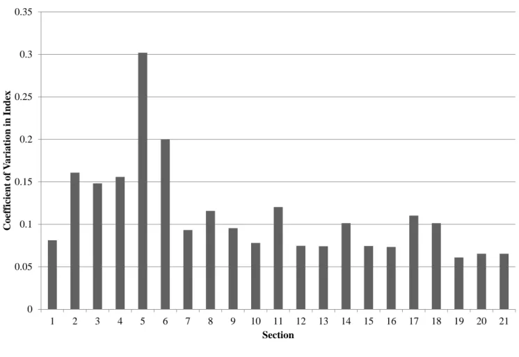
First, Figure 7 and Figure 8 show the average value over time and the coefficient of variation in our IIT stability index, respectively. The index for the agricultural, raw material and light manufacturing sectors are relatively low in average value and high in variation, whereas the index for the machinery sector has high average value and low variation. This indicates that trade in raw material and light manufacturing sectors are likely to be unstable, whereas the machinery trade is more stable. Next, Table 3 shows our estimations with product sector dummies. All country variables are significant, which is consistent with Table 2. In terms of product sector dummies, the coefficients for agricultural, raw material, and light manufacturing sectors appear smaller than those of machinery sectors. This result parallels Figure 7.¹⁶ Therefore, we can conclude that there is substantial variations in IIT stability across sectors, although country factors are still influential.

This sectoral variation helps interpret the country variation in IIT stability index as shown in Table 1. The country pairs with high index values (e.g., pairs including the United States, Germany, France and Japan), are more likely to trade heavy manufacturing products such as machinery that country pairs with low index scores are. Thus, these country pairs have stable IIT. In general, country pairs with stable IIT have large demand and thus are always trading for final products as consumption goods, as well as for

intermediate inputs through foreign direct investment and supply chains. On the other hand, country pairs

14 For example, we tried the following weights and obtained qualitatively similar results: ^{∑ �𝑇𝑇𝑇𝑇𝑇𝑖 𝑖𝑖𝑖𝑖+𝑇𝑇𝑇𝑇𝑇𝑖𝑖𝑖𝑖�}

∑ ∑𝑖 _{𝑖∈Θ𝑖}�𝑇𝑇𝑇𝑇𝑇_{𝑖𝑖𝑖𝑖}+𝑇𝑇𝑇𝑇𝑇_{𝑖𝑖𝑖𝑖}� and

∑ �𝑇𝑇𝑇𝑇𝑇_{𝑖 𝑖𝑖𝑖𝑖}+𝑇𝑇𝑇𝑇𝑇_{𝑖𝑖𝑖𝑖}�

∑ ∑_{𝑖 𝑖∈Ω}�𝑇𝑇𝑇𝑇𝑇_{𝑖𝑖𝑖𝑖}+𝑇𝑇𝑇𝑇𝑇_{𝑖𝑖𝑖𝑖}�.

15 See the appendix A.3. for the 2-digit sector definitions.

16 Even if we split the sample by sector, all results in the product sector estimations are consistent with those of Table 3.

12

with unstable IIT are small and distant countries and tend to specialise more in the trade of food, raw materials and natural resources.¹⁷ The trade in these sectors may be more sensitive to the business cycle, exchange rates and harvest conditions. Importers can purchase these goods in large volume when market conditions are favourable for buyers and keep them as stock, which leads to intermittent imports.

5. C ONCLUSION

This paper reveals that IIT is in fact often unstable when we look at a highly disaggregated level. Some products are traded on a two-way basis in a given year, but then return to one-way trade in subsequent years. This paper introduces the concept of an IIT stability index and finds that country pairs with large markets, high economic development, low exchange rate volatility, geographical proximity, linguistic commonality and shared borders are likely to have stable IIT relationships. Our study also finds variation by product sector in the IIT stability index. Trade in raw material and light manufacturing sectors are more likely to be unstable, whereas machinery trade is more stable.

Lastly, we must mention that there remains room for future research. First of all, our paper is aimed at providing some initial findings on the stability of IIT. Based on our findings, we might be able to

construct a dynamic general equilibrium trade model. One possible way is to extend the method of Eaton et al. (2011). Such a method would allow us to investigate the mechanism of our findings above in more detail, including the dynamic features of stable and unstable IIT. Second, in order to investigate this topic more rigorously, we may extend it to other econometric methodologies, such as time-series analysis using raw trade data instead of the IIT stability index.

R EFERENCES

Albornoz, F., Calvo Pardo, H. F., Corcos, G., and Ornelas, E. (2012). Sequential exporting. Journal of International Economics, 88(1), 17-31.

Arkolakis, C. (2010) Market Penetration Costs and the New Consumers Margin in Inter-national Trade, Journal of Political Economy, 118(6), 1151.1199.

17 For instance, Iceland and New Zealand are both peripheral countries and ranked as unstable IIT countries, as shown in Table1. They export food, raw materials and natural resources as their primary products, which accounts for more than 80%

and 50% of total exports in Iceland and New Zealand, respectively.

13

Aturupane, C., Djankov, S., and Hoekman, B., (1999). Horizontal and Vertical Intra-Industry Trade between Eastern Europe and the European Union.,WeltwirtschaftlichesArchiv/Review of World Economics, 135(1), 62-81.

Azhar, A., Elliott, R., and Milner, C.R., (1998). Static and Dynamic Measurement of Intra-Industry Trade and Adjustment: A Geometric Reappraisal. Weltwirtschaftliches Archiv/Review of World Economics 134 (3): 404–422.

Baldwin, R.E., Forslid, R., Martin, P., Ottaviano, G.P., Robert-Nicoud, F., (2003). Economic Geography and Public Policy. Princeton University Press.

Baldwin, R., and P.Krugman (1989). Persistent Trade Effects of Large Exchange Rate Shocks. The Quarterly Journal of Economics, 104(4), 635-654.

Békés, G., and Muraközy, B. (2012). Temporary trade and heterogeneous firms. Journal of International Economics, 87(2), 232-246.

Bernard, A.B., R.Massari, J-D Reyes and D.Taglioni (2013) “Exporter Dynamics, Firm Size and Growth, and Partial Year Effects”, mimeo.

Besedeš, T. and Prusa, T. (2006) “Ins, outs, and the duration of trade”, Canadian Journal of Economics, Vol. 39, No. 1

Blum, B. S., Claro, S., & Horstmann, I. J. (2013). Occasional and perennial exporters. Journal of International Economics, 90(1), 65-74.

Brülhart, M. (1994). Marginal IIT-Measurement and Relevance for the Pattern of Industrial Adjustment.

Weltwirtschaftliches Archiv/Review of World Economics 30 (3): 600-613.

Brülhart, M. (2009).An Account of Global Intra-industry Trade, 1962-2006., The World Economy, 32(3), 401-459.

Brülhart, M., Elliott R., 2002. Labour Market Effects of Intra-Industry Trade: Evidence for the United Kingdom., Review of World Economics 138 (2): 207-228.

Brulhart, M., Elliott, R. J., & Lindley, J. K. (2006). Intra-industry trade and labour-market adjustment: a reassessment using data on individual workers. Review of World Economics, 142(3), 521-545.

Buono, I., and Fadinger, H., (2012) “The micro dynamics of exporting: Evidence from French firms”, Bank of Italy Termi di Discussione (Working Paper) No. 2012

Cabral, M., and Silva, J. (2006). Intra-industry trade expansion and employment reallocation between sectors and occupations. Review of World Economics, 142(3), 496-520.

DAS, S., ROBERTS, M. J., & TYBOUT, J. R. (2007). MARKET ENTRY COSTS, PRODUCER HETEROGENEITY, AND EXPORT DYNAMICS BY SANGHAMITRA DAS, MARK J. ROBERTS, AND JAMES R. TYBOUT. Econometrica, 75(3), 837-873.

14

Dixit, A. (1989). Hysteresis, import penetration, and exchange rate pass-through. The Quarterly Journal of Economics, 205-228.

Eaton, J., and Kortum, S. (2002). Technology, geography, and trade. Econometrica, 70(5), 1741-1779.

Eaton, J., Kortum, S., and Kramarz, F. (2011). An anatomy of international trade: Evidence from French firms. Econometrica, 79(5), 1453-1498.

Elliott, R and X. Tian (2010a), Sequential Exporting: China as a Launch Pad or Crash Site, mimeo.

Elliott, R and X. Tian (2010b), The Argentinean Connection: Sequential Exporting in the EU, mimeo.

Finicelli, A., Pagano, P., and Sbracia, M. (2013). Ricardian selection. Journal of International Economics, 89(1), 96-109.

Fujita, M., and Thisse, J. F. (2002). Economics of Agglomeration: Cities, Industrial Location, and Regional Growth. Cambridge University Press.

Greenaway, D., R. C. Hine, C. R. Milner, and R. J. R. Elliott (1994). Adjustment and the measurement of marginal intra-industry trade. Weltwirtschaftliches Archiv/Review of World Economics 130 (2): 418 - 427.

Greenaway, D., Hine, R., Milner, C., (1995). Vertical and Horizontal Intra-Industry Trade: A Cross Industry Analysis for the United Kingdom, The Economic Journal, 105, 1505-1518.

Grubel, H. G. and J. P. Lloyd, (1975). Intra-industry Trade: The Theory and Management of International Trade in Differentiated Products (Macmillan, New York).

Hamilton, C., and P. Kniest (1991). Trade Liberalisation, Structural Adjustment and Intra-Industry Trade:

A Note. Weltwirtschaftliches Archiv/Review of World Economics 127 (1): 365 -367.

Helpman, E., and Krugman, P. R. (1985). Market structure and foreign trade: Increasing returns, imperfect competition, and the international economy. MIT press.

Helpman, E., Melitz, M., and Rubinstein, Y. (2008). Estimating Trade Flows: Trading Partners and Trading Volumes. The Quarterly Journal of Economics, 123(2), 441-487.

Impullitti, G., Irarrazabal, A., and Opromolla, L. (2013) “A theory of entry into and exit from export markets”, Journal of International Economics, 90 (2013) 75-90

Jensen, L.and Lüthje, T., (2009). Driving forces of vertical intra-industry trade in Europe 1996-2005., Review of World Economics, 145:469-488.

Krugman, P. (1980). Scale economies, product differentiation, and the pattern of trade. The American Economic Review, 950-959.

Melitz, M. (2003). The Impact of Trade on Intra-Industry Reallocations and Aggregate Industry Productivity, Econometrica, Vol. 71, November 2003, pp. 1695-1725.

Novy, D. (2013). International trade without CES: Estimating translog gravity. Journal of International Economics, 89(2), 271-282.

15

Okubo, T. Picard, P.M and Thisse, J-F (2014). “On the Impact of Competition on Trade and Firm Location”, Journal of Regional Science, 54(5), 731-754.

Ottaviano, G., Tabuchi, T., and Thisse, J.F., (2002). Agglomeration and trade revisited. International Economic Review 43 (2), 409–436.

Papageorgiou, T., & Arkolakis, C. (2009). Learning and Selection into Exporting. In 2009 Meeting Papers (No. 183). Society for Economic Dynamics.

Papke, L.E. and Wooldridge, J.M., (1996). Econometric Methods for Fractional Response Variables with an Application to 401(k) Plan Participation Rates, Journal of Applied Econometrics, 11(6), 619-632.

Ramalho, E.A., Ramalho, J.J.S., and Murteira, J.M.R., (2011). Alternative Estimating and Testing Empirical Strategies for Fractional Regression Models, Journal of Economic Surveys, 25(1), 19-68.

Roberts, M. J., & Tybout, J. R. (1997). The decision to export in Colombia: an empirical model of entry with sunk costs. The American Economic Review, 545-564.

Rose, A., (2000). One money, one market: The effect of common currencies on trade. Economic Policy, April, 9-45.

16

Tables and Figures

Table 1: IIT Stability Index

ISL JPN 0.04 DEU USA 0.99

ISL TUR 0.04 DEU JPN 0.99

CZE ISL 0.05 JPN USA 0.99

ISL ITA 0.06 DEU ITA 0.99

GRC ISL 0.07 DEU FRA 0.98

ISL SVK 0.07 DEU ESP 0.98

HUN ISL 0.09 GBR USA 0.98

GRC MEX 0.10 AUT DEU 0.98

NOR PRT 0.12 ESP FRA 0.98

NZL SVK 0.13 CAN USA 0.98

ISL MEX 0.14 FRA ITA 0.98

NZL TUR 0.14 KOR USA 0.98

ISL KOR 0.14 GBR JPN 0.98

HKG POL 0.15 FRA USA 0.98

GRC SVK 0.15 DEU DNK 0.98

AUT ISL 0.15 ESP ITA 0.97

GRC KOR 0.16 AUT ITA 0.97

AUS TUR 0.16 CZE DEU 0.97

ISL POL 0.17 DEU HUN 0.97

IRL ISL 0.17 HKG USA 0.97

ISL NZL 0.18 DEU GBR 0.97

CZE NZL 0.18 ITA USA 0.97

HUN NZL 0.19 GBR ITA 0.97

AUS SVK 0.19 FRA JPN 0.97

GRC NZL 0.20 GBR IRL 0.97

Top 25 Unstable Pairs Top 25 Stable Pairs

17 Table 2: Estimation Results

(I) (II) (III)

Method OLS Fractional OLS

GDP Product 0.003*** 0.003*** 0.002***

[0.000] [0.000] [0.000]

GDP Capita Product 0.006*** 0.006*** 0.004***

[0.001] [0.001] [0.000]

Distance -0.087*** -0.080*** -0.071***

[0.008] [0.007] [0.000]

Language 0.136*** 0.162*** 0.077***

[0.028] [0.029] [0.001]

Contiguity 0.015 0.113** 0.201***

[0.038] [0.051] [0.001]

Volatility -0.130*** -0.143*** -0.044***

[0.050] [0.045] [0.001]

Aggregation Total Total HS6

Observations 378 378 1,903,986

R-squared 0.5900 0.4988

Log pseudolikelihood -142

Notes: Robust standard error in brackets. ***, **, and * indicate significance at the 1%, 5%, and 10% levels, respectively.

We report marginal effects for the fractional-logit model. Observations are defined at a country-pair level in columns (I) and (II) and at a country-pair 6-digit HS category level in column (III). In column (III), we include 6-digit HS category level fixed effects.

18

Table 3: Estimation Results with Product Sector Dummy Variables

Coef. R.S.E. Coef. R.S.E.

GDP Product 0.003*** [0.000] 0.003*** [0.000]

GDP Capita Product 0.007*** [0.000] 0.007*** [0.000]

Distance -0.103*** [0.002] -0.100*** [0.002]

Language 0.139*** [0.009] 0.150*** [0.009]

Contiguity 0.100*** [0.012] 0.166*** [0.015]

Volatility -0.029** [0.014] -0.030** [0.014]

Live animals -1.839*** [0.044] -2.336*** [0.041]

Vegetable products -1.848*** [0.044] -2.345*** [0.041]

Animal/vegetable fats and oils -1.983*** [0.044] -2.494*** [0.041]

Food products -1.669*** [0.044] -2.175*** [0.041]

Mineral products -1.919*** [0.044] -2.419*** [0.041]

Chemical products -1.607*** [0.044] -2.117*** [0.041]

Plastics and rubber -1.485*** [0.044] -1.991*** [0.041]

Leather products -1.672*** [0.044] -2.179*** [0.041]

Wood products -1.750*** [0.045] -2.251*** [0.041]

Paper products -1.570*** [0.044] -2.081*** [0.041]

Textiles -1.666*** [0.044] -2.173*** [0.041]

Footwear -1.670*** [0.045] -2.177*** [0.041]

Plastic or glass products -1.684*** [0.044] -2.190*** [0.041]

Precision metals -1.758*** [0.045] -2.259*** [0.041]

Base Metal -1.613*** [0.044] -2.123*** [0.040]

Machinery -1.488*** [0.044] -1.995*** [0.041]

Transport equipment -1.656*** [0.045] -2.164*** [0.041]

Precision machinery -1.551*** [0.044] -2.062*** [0.041]

Arms and ammunition -1.974*** [0.044] -2.483*** [0.041]

Miscellaneous -1.562*** [0.045] -2.073*** [0.041]

Art products -1.778*** [0.045] -2.277*** [0.041]

Observations 7,938 7,938

R-squared 0.8828

Log pseudolikelihood -3066

OLS Fractional

Notes: “S.E.” indicates robust standard errors. ***, **, and * indicate significance at the 1%, 5%, and 10% levels, respectively. Observations are defined at a country-pair-section level. We report marginal effects for the fractional-logit model.

19

Figure 1: Trend in IIT Index, Simple Average of All Countries

0.00 0.02 0.04 0.06 0.08 0.10 0.12 0.14 0.16 0.18

1994 1995 1996 1997 1998 1999 2000 2001 2002 2003 2004 2005 2006 2007 2008 2009 2010

IIT Index

Year

20 Figure 2: Years of Two-way Trade, 1994–2010

51%

7%

4% 4% 3% 3% 2% 2% 2% 2% 2% 2% 1% 2% 2% 2% 2%

11%

0 500,000 1,000,000 1,500,000 2,000,000 2,500,000

0 1 2 3 4 5 6 7 8 9 10 11 12 13 14 15 16 17

Number of Observations

Number of IIT Years

21

Figure 3: Years of Two-way Trade, 1994–2010 (Excluding zero trade)

46%

15%

7%

5% 3% 2% 2% 1% 1% 1% 1% 1% 1% 1% 1% 1%

11%

0 200,000 400,000 600,000 800,000 1,000,000 1,200,000 1,400,000 1,600,000 1,800,000 2,000,000

1 2 3 4 5 6 7 8 9 10 11 12 13 14 15 16 17

Number of Observations

Number of IIT Consecutive Years

22

Figure 4: Plot of Trade Values

(Import or export value, whichever is smaller)

23 Figure 5: IIT and Stability Index

0.0 0.1 0.2 0.3 0.4 0.5 0.6 0.7 0.8 0.9 1.0

0 10,000 20,000 30,000 40,000 50,000 60,000 70,000 80,000

Stability Index

Number of IIT

24

Figure 6: Comparison of Estimation Results for Annual Trade versus Two-year Trade Data

y = 0.8962x R² = 0.8937

0 0.1 0.2 0.3 0.4 0.5 0.6 0.7 0.8 0.9 1

0 0.1 0.2 0.3 0.4 0.5 0.6 0.7 0.8 0.9 1

Stability Index Based on Annual Data

Stability Index Based on Biannual Data

25

Figure 7: Average Index Value Over Time by Product Sector

0 0.05 0.1 0.15 0.2 0.25

1 2 3 4 5 6 7 8 9 10 11 12 13 14 15 16 17 18 19 20 21

Over-time Average Index

Section

26

Figure 8: Coefficient of Variation in Index by Product Sector

0 0.05 0.1 0.15 0.2 0.25 0.3 0.35

1 2 3 4 5 6 7 8 9 10 11 12 13 14 15 16 17 18 19 20 21

Coefficient of Variation in Index

Section

A.1. A simple numerical example for the scoring rule in Section 3.

Stability of IIT statu s

1995 1996 1997 1998 1999 2000 2001 2002 2003 2004 Score IIT stability index

Case 1 IIT IIT IIT IIT IIT IIT IIT IIT IIT IIT 55 1

Case 2 IIT One-way One-way One-way One-way One-way One-way One-way One-way One-way 1 0.018 Case 3 One-way IIT One-way One-way One-way One-way One-way One-way One-way One-way 1 0.018

Case 4 IIT One-way IIT IIT IIT IIT IIT IIT IIT IIT 37 0.673

Case 5 One-way One-way One-way One-way One-way One-way One-way One-way One-way One-way 0 0.000 Case 6 IIT One-way IIT One-way One-way One-way One-way One-way One-way One-way 2 0.036

Case 7 IIT IIT IIT One-way IIT IIT IIT One-way One-way IIT 13 0.236

Case 8 One-way IIT One-way IIT One-way IIT One-way IIT One-way IIT 5 0.091

For consecutive IIT, the number of years of consecutive IIT entry is added. For the case 1, the total score is computed as 1+2+3+4+5+6+7+8+9+10=55 For case 2, and 3, the score is 1 because IIT is recorded only once. For case 4, the total score is 1+0+1+2+3+4+5+6+7+8=37

To confine the index into the support of 0-1, the total score is divided by 55 (the maximum possible score).

Variable Obs Mean Std. Dev. Min Max

Stability 378 0.6845 0.2528 0.0409 0.9910

GDP Product 378 708.0380 53.8553 562.5572 872.5188

GDP Capita Product 378 98.7631 8.0817 76.6462 113.8035

Distance 378 8.1462 1.1443 4.0879 9.8826

Language 378 0.0899 0.2865 0 1

Contiguity 378 0.0635 0.2442 0 1

Volatility 378 0.1651 0.1737 0.0100 0.7150

29 A.3. Product Sector Tariff Code

Section Description

1 Live animals ; animal products 2 Vegetable products

3 Animal or vegetable fats and oils and their cleavage products;prepared edible fats ; animal or vegetable waxes

4 Prepared foodstuffs ; beverages, spirits and vinegar ; tabacco and manufactured tabacco substitutes

5 Mineral products

6 Products of the chemical or allied industries

7 Plastics and articles thereof ; rubber and articles thereof

8 Raw hides and skins, leather, furskins and articles thereof ; saddlery and harness ; travel goods, handbags and similar containers ; articles of animal gut (other than silkworm gut) 9 Wood and articles of wood ; wood charcoal ; cork and articles of cork ; manufactures

of straw, of esparto or of other plaiting materials ; basketware and wickerwork 10 Pulp of wood or of other fibrous cellulosic materials ; waste and scrap of paper or

paperboard ; paper and paperboard and articles thereof 11 Textiles and texitile articles

12 Footwear, headgear umbrellas, sun umbrellas, walking-sticks, seatstics, whips, riding- crops and parts thereof ; prepared feathers and articles made therewith ; artificical flowers ; articles of human hair

13 Articles of stone, plaster, cement, asbestos, mica or similar materials ; ceramic products

; glass and glassware

14 Natural or cultured pearls, precious or semi-precious stones, precious metals, metals clad with precious metal, and articles thereof ; imitation jewellery ; coin

15 Base metals and articles of base metal

16 Machinery and mechanical appliances ; electorical equipment ; parts thereof ; sound recorders and reproducers, television image and sound recorders and reproducers, and parts and accessories of such articles

17 Vehicicles, aircraft, vessels and associated transport equipment

18 Optical, photographic, cinematographic, mesuring, checking, precision, medical or surgical instruments and apparatus ; clocks and watches ; musical instruments ; parts and accessories thereof

19 Arms and ammunition ; parts and accessories thereof 20 Miscellaneous manufactured articles

21 Works of art, collectors'' pieces and antiques