Quantifying Dynamic Leakage

PAPER

Quantifying Dynamic Leakage

– Complexity Analysis and Model Counting-based Calculation –

Bao Trung CHU^†a),Nonmember, Kenji HASHIMOTO^†,Member,andHiroyuki SEKI^†,Fellow

SUMMARY A program is non-interferent if it leaks no secret infor- mation to an observable output. However, non-interference is too strict in many practical cases and quantitative information flow (QIF) has been proposed and studied in depth. Originally, QIF is defined as the average of leakage amount of secret information over all executions of a program.

However, a vulnerable program that has executions leaking the whole se- cret but has the small average leakage could be considered as secure. This counter-intuition raises a need for a new definition of information leakage of a particular run,i.e., dynamic leakage. As discussed in[5], entropy- based definitions do not work well for quantifying information leakage dy- namically; Belief-based definition on the other hand is appropriate for de- terministic programs, however, it is not appropriate for probabilistic ones.

In this paper, we propose new simple notions of dynamic leakage based on entropy which are compatible with existing QIF definitions for deterministic programs, and yet reasonable for probabilistic programs in the sense of[5]. We also investigated the complexity of computing the pro- posed dynamic leakage for three classes of Boolean programs. We also implemented a tool for QIF calculation using model counting tools for Boolean formulae. Experimental results on popular benchmarks of QIF research show the flexibility of our framework. Finally, we discuss the im- provement of performance and scalability of the proposed method as well as an extension to more general cases.

key words:quantitative information flow, hybrid monitor, dynamic leakage

1. Introduction

Researchers have realized the importance of knowing where confidential information reaches by the execution of a pro- gram to verify whether the program is safe. The non- interferenceproperty, namely, any change of confidential input does not affect public output, was coined in 1982 by Goguen and Meseguer[14]as a criterion for the safety.

This property, however, is too strict in many practical cases, such as password verification, voting protocol and averaging scores. A more elaborated notion called quantitative infor- mation flow (QIF)[23]has been getting much attention of the community. QIF is defined as the amount of information leaking from secret input to observable output. The pro- gram can be considered to be safe (resp. vulnerable) if this quantity is negligible (resp. large). QIF analysis is not easier than verifying non-interference property because if we can calculate QIF of a program, we can decide whether it sat- isfies non-interference or not. QIF calculation is normally approached in an information-theoretic fashion to consider a program as a communication channel with input as source,

Manuscript received May 15, 2019.

Manuscript publicized July 11, 2019.

†The authors are with Nagoya University, Nagoya-shi, 464–

0814 Japan.

a) E-mail: [email protected] DOI: 10.1587/transinf.2019EDP7132

and output as destination. The quantification is based on en- tropy notions including Shannon entropy, min-entropy and guessing entropy[23]. QIF (or the information leakage) is defined as the remaining uncertainty about secret input af- ter observing public output, i.e., the mutual information be- tween source and destination of the channel. Another quan- tification proposed by Clarkson, et al.[11], is the difference between ‘distances’ (Kullback-Leibler divergence) from the probability distribution on secret input that an attacker be- lieves in to the real distribution, before and after observing the output values.

While QIF is about the average amount of leaked in- formation over all observable outputs, dynamic leakage is about the amount of information leaked by observing apar- ticularoutput. Hence, QIF is aimed to verify the safety of a program in a static scenario in compile time, and dynamic leakage is aimed to verify the safety of a specific running of a program. So which of them should be used as a metric to evaluate a system depends on in what scenario the software is being considered.

Example 1.1:

ifsource<16 thenout put←8+source elseout put←8

In Example 1.1 above, assume sourceto be a positive in- teger, then there are 16 possible values ofout put, from 8 to 23. While an observable value between 9 and 23 reveals everythingabout the secret variable, i.e., there is only one possible value of source to produce such out put, a value of 8 gives almost nothing, i.e., there are so many possible values of source which produce 8 as output. Taking the average of leakages on all possible execution paths results in a relatively small value, which misleads us into regard- ing that the vulnerability of this program is small. There- fore, it is crucial to differentiate risky execution paths from safe ones by calculating dynamic leakage, i.e., the amount of information that can be learned from observing the out- put which is produced by a specific execution path. But, as discussed in[5], any of existing QIF models (either entropy based or belief tracking based) does not always seem rea- sonable to quantify dynamic leakage. For example, entropy- based measures give sometimes negative leakage. Usually, we consider that the larger the value of the measure is, the more information is leaked, and in particular, no informa- tion is leaked when the value is 0. In the interpretation, it is not clear how we should interpret a negative value as a leak- age metric. Actually,[5]claims that the non-negativeness is Copyright c2019 The Institute of Electronics, Information and Communication Engineers

a requirement for a measure of dynamic QIF. Also,MONO, one of the axioms for QIF in[2] turns out to be identical to this non-negative requirement. Belief-based one always give non-negative leakage for deterministic programs but it may become negative for probabilistic programs. In addi- tion, the measure using belief model depends on secret val- ues. This would imply (1) even if a same output value is ob- served, the QIF may become different depending on which value is assumed to be secret, which is unnatural, and (2) a side-channel may exist when further processing is added by system managers after getting quantification result. Hence, as suggested in[5], it is better to introduce a new notion for quantifying dynamic leakage caused by observing a specific output value.

The contributions of this paper are three-fold.

• We present our criteria for an appropriate definition of dynamic leakage and propose two notions that satisfy those criteria. We propose two notions because there is a trade-offbetween the easiness of calculation and the preciseness (see Sect. 2).

• Complexity of computing the proposed dynamic leak- ages is analyzed for three classes of Boolean programs.

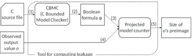
• By applying model counting of logical formulae, a pro- totype was implemented and feasibility of computing those leakages is discussed based on experimental re- sults.

According to [5], we arrange three criteria that a ‘good’

definition of dynamic leakage should satisfy, namely, the measure should be (R1) non-negative, (R2) independent of a secret value to prevent a side channel and (R3) compat- ible with existing notions to keep the consistency within QIF as a whole (both dynamic leakage and normal QIF).

Based on those criteria, we come up with two notions of dynamic leakage QIF1 and QIF2, where both of them sat- isfy all (R1), (R2) and (R3). QIF1, motivated by entropy- based approach, takes the difference between the initial and remaining self-information of the secret before and after ob- serving output as dynamic leakage. On the other hand, QIF2 models that of the joint probability between secret and out- put. Because both of them are useful in different scenar- ios, we studied these two models in parallel in the theoret- ical part of the paper. We call the problems of computing QIF1 and QIF2 for Boolean programs CompQIF1 and Com- pQIF2, respectively. For example, we show that even for deterministic loop-free programs with uniformly distributed input, both CompQIF1 and CompQIF2 areP-hard. Next, we assume that secret inputs of a program are uniformly distributed and consider the following method of computing QIF1 and QIF2 (only for deterministic programs for QIF2 by the technical reason mentioned in Sect. 4): (1) translate a program into a Boolean formula that represents relation- ship among values of variables during a program execution, (2) augment additional constraints that assign observed out- put values to the corresponding variables in the formula, (3) count models of the augmented Boolean formula projected on secret variables, and (4) calculate the necessary probabil-

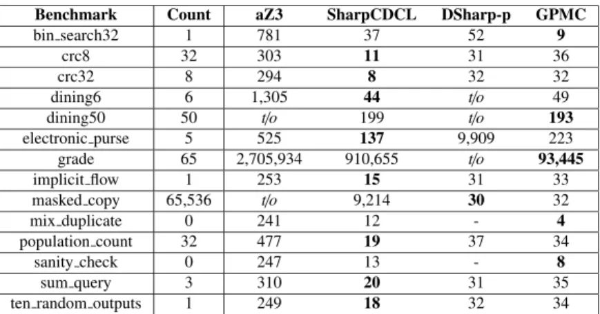
ity and dynamic leakage using the counting result. Based on this method, we conducted experiments using our prototype tool with benchmarks taken from QIF related literatures, in which programs are deterministic, to examine the feasibil- ity of automatic calculation. We also give discussion, in Sect. 5.3, on difficulties and possibilities to deal with more general cases, such as, of probabilistic programs. In step (3), we can flexibly use any off-the-shelf model counter. To investigate the scalability of this method, we used four state- of-the-art counters, SharpCDCL[15]and GPMC[24],[32]

for SAT-based counting, an improved version of aZ3[22]

for SMT-based counting, and DSharp-p[20],[30]for SAT- based counting in d-DNNF fashion. Finally, we discuss the feasibility of automatic calculation of the leakage in general case.

Related workThe very early work oncomputational com- plexity of QIF is that of Yasuoka and Terauchi. They proved that even the problem of comparing QIF of two pro- grams, which is obviously not more difficult than calculat- ing QIF, is not a k-safety property for any k[27]. Conse- quently, self-composition, a successful technique to verify non-interference property, is not applicable to the compar- ison problem. Their subsequent work[28]proves a similar result for bounding QIF, as well as thePP-hardness of pre- cisely quantifying QIF in all entropy-based definitions for loop-free Boolean programs. Chadha and Ummels[9]show that the QIF bounding problem of recursive programs is not harder than checking reachability for those programs. De- spite given those evidences about the hardness of calculating QIF, for this decade,precise QIF analysisgathers much at- tention of the researchers. In [15], Klebanov et al. reduce QIF calculation toSAT problem projected on a specific set of variables as a very first attempt to tackle with automat- ing QIF calculation. On the other hand, Phan et al. re- duce QIF calculation toSMT problem for utilizing existing SMT (satisfiability modulo theory) solvers. Recently, Val et al.[25]reported a method that can scale to programs of 10,000 lines of code but still based on SAT solver and sym- bolic execution. However, there is still a gap between such improvements and practical use, and researchers also work onapproximating QIF. K¨opf and Rybalchenko[16]propose approximated QIF computation by sandwiching the precise QIF by lower and upper bounds using randomization and abstraction, respectively with a provable confidence. Leak- Watch of Chothia et al.[10], also gives approximation with provable confidence by executing a program multiple times.

Its descendant called HyLeak[7]combines the randomiza- tion strategy of its ancestor with precise analysis. Also using randomization but in Markov Chain Monte Carlo (MCMC) manner, Biondi et al.[6] utilize ApproxMC2, an existing model counter created by some of the co-authors. Ap- proxMC2 provides approximation on the number of models of a Boolean formula in CNF with adjustable precision and confidence. ApproxMC2 uses hashing technique to divide the solution space into smaller buckets with almost equal number of elements, then counts the models for only one

bucket and multiplies it by the number of buckets. As for dynamic leakage, McCamant et al.[17]consider QIF as net- work flow through programs and propose a dynamic anal- ysis method that can work with executable files. Though this model can scale to very large programs, its precision is relatively not high. Alvim et al.[2]give some axioms for a reasonable definition of QIF to satisfy and discuss whether some definitions of QIF satisfy the axioms. Note that these axioms are forstaticQIF measures, which differ from dy- namic leakage. However, given a similarity between static and dynamic notions, we investigated how our new dynamic notions fit in the lens of the axioms (refer to Sect. 2).

Dynamic information flow analysis (or taint analysis) is a bit confusing term that does not mean an analysis of dy- namic leakage, but a runtime analysis of information flow.

Dynamic analysis can abort a program as soon as an unsafe information flow is detected. Also, hybrid analysis has been proposed for improving dynamic analysis that may abort a program too early or unnecessarily. In hybrid analysis, the unexecuted branches of a program is statically analyzed in parallel with the executed branch. Among them, Bielova et al.[4]define the knowledgeκ(z) of a program variablezas the information on secret that can be inferred fromz(techni- cally,κ(z)⁻¹(v) is the same of the pre-image of an observed valuev of z, defined in Sect. 2). In words, hybrid analy- sis updates the ‘dynamic leakage’ under the assumption that the program may terminate at each moment. Our method is close to[4]in the sense that the knowledge κ(z)⁻¹(v) is computed. The difference is that we conduct the analysis after the a program is terminated andvis given. We think this is not a disadvantage compared with hybrid analysis be- cause the amount of dynamic leakage of a program is not determined until a program terminates in general.

Structure of the remaining parts: Sect. 2 is dedicated to introduce new notions, i.e., QIF1 and QIF2, of dynamic leakage and some properties of them. The computational complexity of CompQIF1 and CompQIF2 is discussed in Sect. 3. Section 4 gives details on calculating dynamic leak- age based on model counting. Experimental results and dis- cussion are provided in Sect. 5 and the paper is concluded in Sect. 6.

2. New Notions for Dynamic Leakage

2.1 QIF₁and QIF₂

The standard notion for static quantitative information flow (QIF) is defined as the mutual information between random variablesS for secret input andOfor observable output:

QIF=H(S)−H(S|O) (1)

whereH(S) is the entropy ofS andH(S|O) is the expected value ofH(S|o), which is the conditional entropy ofS when observing an outputo. Shannon entropy and min-entropy are often used as the definition of entropy, and in either case, H(S)−H(S|O)≥0 always holds by the definition.

In[5], the author discusses the appropriateness of the existing measures for dynamic QIF and points out their drawbacks, especially, each of these measures may become negative. Hereafter, letSandOdenote the finite sets of in- put values and output values, respectively. SinceH(S|O)=

o∈Op(o)H(S|o), [5] assumes the following measure ob- tained by replacingH(S|O) withH(S|o) in (1) for dynamic QIF:

QIF^dyn(o)=H(S)−H(S|o). (2) However, QIF^dyn(o) may become negative even if a program is deterministic (see Example 2.1). Another definition of dynamic QIF is proposed in[11]as

QIF^{belie f}( ˙s,o)=DKL(ps_˙||pS)−DKL(ps_˙||pS|o) (3) where DKL is KL-divergence defined as DKL(p||q) =

s∈Sp(s) log_q(^p(s)_s), and ps_˙(s)=1 ifs=s˙andps_˙(s)=0 oth- erwise. Intuitively, QIF^{belie f}( ˙s,o) represents how closer the belief of an attacker approaches to the secret ˙sby observing o. For deterministic programs, QIF^{belie f}( ˙s,o)=−logp(o)≥ 0[5]. However, QIF^{belie f} may still become negative if a pro- gram is probabilistic (see Example 2.2).

Let Pbe a program with secret input variable S and observable output variable O. For notational convenience, we identify the names of program variables with the corre- sponding random variables. Throughout the paper, we as- sume that a program always terminates. The syntax and se- mantics of programs assumed in this paper will be given in the next section. For s ∈ Sand o ∈ O, let pS O(s,o), pO|S(o|s), pS|O(s|o), pS(s),pO(o) denote the joint probabil- ity ofs∈ Sando∈ O, the conditional probability ofo∈ O givens ∈ S(the likelihood), the conditional probability of s∈ Sgiveno ∈ O(the posterior probability), the marginal probability ofs∈ S(the prior probability) and the marginal probability ofo ∈ O, respectively. We often omit the sub- scripts asp(s,o) andp(o|s) if they are clear from the context.

By definition,

p(s,o)=p(s|o)p(o)=p(o|s)p(s), (4) p(o)=

s∈S

p(s,o), (5)

p(s)=

o∈O

p(s,o). (6)

We assume that (the source code of)Pand the prior proba- bilityp(s) (s∈ S) are known to an attacker. Foro ∈ O, let pre_P(o)={s∈ S |p(s|o)>0}, which is called the pre-image ofo(by the programP).

Considering the discussions in the literature, we aim to define new notions for dynamic QIF that satisfy the follow- ing requirements:

(R1) Dynamic QIF should be always non-negative because an attacker obtains some information (although some- times very small or even zero) when he observes an output of the program.

(R2) It is desirable that dynamic QIF is independent of a

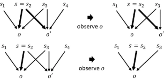
Fig. 1 QIF1(the upper) and QIF2(the lower)

secret input s ∈ S. Otherwise, the controller of the system may change the behavior for protection based on the estimated amount of the leakage that depends ons, which may be a side channel for an attacker.

(R3) The new notion should be compatible with the exist- ing notions when we restrict ourselves to special cases such as deterministic programs, uniformly distributed inputs, and taking the expected value.

The first proposed notion is the self-information of the se- cret inputs consistent with an observed outputo∈ O. Equiv- alently, the attacker can narrow down the possible secret in- puts after observingoto the pre-image ofoby the program.

We consider the self-information ofs∈ Safter the observa- tion as the logarithm of the probability ofsdivided by the sum of the probabilities of the inputs in the pre-image ofo (see the upper part of Fig. 1).

QIF₁(o)=−log(

s∈pre_P(o)

p(s)). (7)

The second notion is the self-information of the joint events s ∈ Sand an observed outputo∈ O(see the lower part of Fig. 1). This is equal to the self-information ofo.

QIF₂(o)=−log(

s∈S

p(s,o)) (8)

=−logp(o)=−logp(s,o)+logp(s|o). (9) Both notions are defined by considering how much possi- ble secret input values are reduced by observing an output.

We propose two notions because there is a trade-offbetween the easiness of calculation and the appropriateness. As il- lustrated in Example 2.2, QIF₂ can represent the dynamic leakage more appropriately than QIF₁ in some cases. On the other hand, the calculation of QIF₁is easier than QIF₂ as discussed in Sect. 4. Both notions are independent of the secret inputs∈ S(Requirement (R2)).

0≤QIF₁(o)≤QIF₂(o). (10)

If we assume Shannon entropy, QIF=−

s∈S

p(s) logp(s)

+

o∈O

p(o)

s∈S

p(s|o) logp(s|o) (11)

=−

s∈S

p(s) logp(s)

+

s∈S,o∈O

p(s,o) logp(s|o). (12)

If a program is deterministic, for eachs∈ S, there is exactly oneos ∈ Osuch that p(s,os) = p(s) and p(s,o) = 0 for oos, and therefore

QIF=

s∈S,o∈O

p(s,o)(−logp(s,o)+logp(s|o)). (13) Comparing (9) and (13), we see that QIF is the expected value of QIF₂, which suggests the compatibility of QIF₂ with QIF (Requirement (R3)) when a program is determin- istic. Also, if a program is deterministic, QIF^{belie f}( ˙s,o) =

−logp(o), which coincides with QIF₂(o) (Requirement (R3)). By (10), Requirement (R1) is satisfied. Also in (10), QIF₁(o)=QIF₂(o) holds for everyo∈ Oif and only if the program is deterministic.

Theorem 2.1: If a program P is deterministic, for every o∈ Oands∈ S,

QIF^{belie f}(s,o)=QIF₁(o)=QIF₂(o)=−logp(o).

If input values are uniformly distributed, QIF₁(o) = log_|pre^|S|_P(o)|for everyo∈ O.

Let us get back to the Example 1.1 in the previous sec- tion to see how new notions convey the intuitive meaning of dynamic leakage. We assume: bothsourceandout putare 8-bit numbers of which values are in 0..255, sourceis uni- formly distributed over this range. Then, because the pro- gram in this example is deterministic, as mentioned above QIF₁ coincides with QIF₂. We have QIF₁(out put = 8) =

−log²⁴¹₂₅₆=0.087bitswhile QIF₁(out put=o)=−log₂₅₆¹ = 8bitsfor every obetween 9 and 23. This result addresses well the problem of failing to differentiate vulnerable output from safe ones of QIF.

Example 2.1: Consider the following program taken from Example 1 of[5]:

ifS =s1thenO←aelseO←b

Assume that the probabilities of inputs are p(s1) = 0.875, p(s₂) = 0.0625 and p(s₃) = 0.0625. Then, we have the following output and posterior probabilities:

p(a)=0.875,p(b)=0.125 p(s1|a)=1,p(s2|a)=p(s3|a)=0 p(s₁|b)=0,p(s₂|b)=p(s₃|b)=0.5

If we use Shannon entropy, H(S) = 0.67, H(S|a) = 0 and H(S|b) = 1. Thus, QIF^dyn(b) = −0.33, which is negative as pointed out in [5]. Also, QIF₂(a) =

−logp(a)=−log 0.875=0.19 and QIF₂(b)=−logp(b)=

−log 0.125=3. QIF₂(a)<QIF₂(b) reflects the fact that the difference of the posterior and the prior of each input when observingbis larger (s1: 0.875→0,s2,s3: 0.0625→0.5) than observinga(s1: 0.875→1,s2,s3: 0.0625→0).

Since the program is deterministic, QIF^{belie f}(s,o) = QIF₁(o)=QIF₂(o).

o a b QIF^dyn(o) 0.67 −0.33

QIF₂(o) 0.19 3

Example 2.2: The next program is quoted from Example 2 of[5]wherec₁r[]₁₋r c₂means that the program chooses c1with probabilityrandc2with probability 1−r.

ifS =s₁thenO←a_0.81[]_0.19O←b elseO←a_0.09[]_0.91O←b

Assume that the probabilities of inputs arep(s1)=0.25 and p(s2) = 0.75. (p(a),p(b)) = (0.25,0.75)

0.81 0.19 0.09 0.91

= (0.27,0.73) and the posterior probabilities are calculated by (4) as:

p(s₁|a)=0.75,p(s₂|a)=0.25 p(s1|b)=0.065,p(s2|b)=0.935

Let us use Shannon entropy for QIF^dyn. As H(S) = H(S|a)=−0.25 log 0.25−0.75 log 0.75, QIF^dyn(a)=H(S)−

H(S|a) = 0. As already discussed in [5], QIF^dyn(a) = 0 though an attacker may think thatS = s1 is more proba- ble by observingO=a. For eacho∈ {a,b}, QIF^{belie f}(s,o) takes different values (one of them is negative) depending on whether s = s₁ or s₂ is the secret input. QIF₂(a) =

−logp(a)=−log 0.27=1.89 and QIF2(b)=−logp(b)=

−log 0.73 =0.45. QIF₁(a) =QIF₁(b) =0 because the set of possible input values does not shrink whichevera or b is observed. Similarly to Example 2.1, QIF₂(a) >QIF₂(b) reflects the fact that the probability of each input when ob- serving a varies more largely (s1 : 0.25 → 0.75, s2 : 0.75 → 0.25) than when observingb(s1 : 0.25 → 0.065, s2: 0.75→0.935). In this example, the number|S|of input values is just two, but in general,|S|is larger and we can expect|preP(o)|is much smaller than|S|and QIF₁serves a better measure for dynamic QIF.

o a b

QIF^dyn(o) 0 0.46 QIF^{belie f}(s1,o) 1.58 −1.94 QIF^{belie f}(s₂,o) −1.58 0.32

QIF₁(o) 0 0

QIF₂(o) 1.89 0.45

A program isnon-interferentif for everyo ∈ Osuch that p(o) > 0 and for every s ∈ S, p(o) = p(o|s). Assume a programPis non-interferent. By (4), p(s) = p(s|o) for everyo ∈ O(p(o)>0) ands∈ S, then QIF=0 by (11). If Pis deterministic in addition,p(o)= p(o|s)=1 foro∈ O (p(o)>0) ands∈ S. That is, if a program is deterministic and non-interferent, it has exactly one possible output value.

Relationship to the hybrid monitor Let us see how our notions relate to the knowledge tracking hybrid monitor pro- posed by Bielova et al.[4].

Example 2.3: Consider the following program taken from Program 5 of[4]:

ifhthenz←x+y elsez←y-x;

outputz

wherehis a secret input,xandyare public inputs andzis a public output.

In [4], the knowledge about secret input hcarried by public outputzisκ(z)=λρ.if([[h]]_ρ,[[x+y]]_ρ,[[y−x]]_ρ) where ρis an initial environment (an assignment of values to h, x andy) and [[e]]_ρ is the evaluation ofein ρ. If h = 1, x = 0 and y = 1, thenz = 1. In[4], to verify whether this value ofzreveals any information abouthin this setting of public inputs (i.e., x =0, y = 1), they takeκ(z)⁻¹(1) = {ρ|if([[h]]_ρ,[[x+y]]ρ,[[y−x]]_ρ)=1}={ρ|if([[h]]_ρ,1,1)=1}.

Becauseif([[h]]_ρ,1,1) = 1 for everyρ,[4] concluded that z=1 in that setting leaks no information.

On the other hand, with that settings of x = 0 and y = 1, givenz =1 as the observed output, hcan be either trueor f alse. For the program is deterministic, QIF₁(z = 1) = QIF₂(z = 1) = −log

p(s|o)>0p(s) = −log(p(h = true)+p(h = f alse)) = −log 1 = 0, which is consistent with that of[4]though the approach looks different. Actu- ally, the functionκ(z) encodes all information revealed from a value ofzabout secret input. By applyingκ(z)⁻¹for a spe- cific valueoofz, we get the pre-image ofo. In other words, κ(z)⁻¹(o) is exactly what we are getting toward quantifying our notions of dynamic leakage. The monitor proposed in [4] tracks the knowledge about secret input carried by all variables along an execution of a program according to the inlined operational semantics. It seems, however, impracti- cal to store all the knowledge during an execution, and fur- thermore, it would take time to compute the inverse of the knowledge when an observed output is fixed.

2.2 An Axiomatic Perspective

The three requirements (R1), (R2) and (R3) we presented summarize the intuitions about dynamic leakage following the spirit of[5]. However, those requirements lack a firm back-up theory, whilst in [2]Alvim et al. provide a set of axioms for QIF. Despite there is difference between QIF and dynamic leakage, we investigate in this subsection how well our notions fit in the lens of those axioms to confirm their feasibility to be used as a metric.

2.2.1 Preliminaries

This subsection briefly summarizes the background theory of[2]to make this paper self-contained. Following the no- tation in Sect. 2.1, letPbe a program with secret input vari- able S and observable output variable Oand let SandO denote the sets of input values and output values, respec- tively. We denote a prior distribution overSbyπjust for readability in this subsection. LetDXdenote the set of all

probability distributions over a finite setX. Theprior vul- nerabilityV : DS → R(R is the set of reals) is defined based on the type of threat which is considered in the con- text. For instance, we may defineBayesprior vulnerability Vb(π)=maxs∈Sπ(s).

A hyper-distribution (abbrev. hyper) over a finite set Xis a distribution on distributions onX. Thus, the set of all hypers overXisD(DX), which is abbreviated asD²X.

A programP transforms a prior distributionπ ∈ DS to a collection of posterior distributionsp(s|o) (as a function that takess ∈ Sas an argument) with probability p(o). Hence, Pcan be regarded as a mapping from DStoD²S. Then, theposterior vulnerabilityV : D²S → Ris defined either as the expected value (E xp_ΔV) or as the maximum value (max _ΔV) of the prior vulnerability over a hyperΔ∈D²S, in which Δdenotes the set of posterior distribution with non-zero probability. We use [π] to denote the point-hyper assigning probability 1 toπ, and [π,P] to denote the hyper obtained by the action ofPonπ.

In [2], three axioms for prior vulnerability and three axioms for posterior vulnerability are proposed.

For prior vulnerability,

Continuity (CNTY):∀π.Vis a continuous function ofπ;

Convexity (CVX):∀

iaiπⁱ.V(

iaiπⁱ)≤

iaiV(πⁱ); and Quasiconvexity (Q-CVX):∀

iaiπⁱ.V(

iaiπⁱ)≤maxiV(πⁱ), providedaiare non-negative real numbers adding up to 1.

For posterior vulnerability, Non-interference (NI):∀π.V[π] =V(π);

Data-processing inequality (DPI):

∀π,P,Q.V[π, P]≥V[π,PQ]; and

Monotonicity (MONO):∀π,P : V[π,P] ≥ V(π), provided P,Qare programs, andPQdenotes the sequential composi- tion ofPandQin this order.

2.2.2 Fit in the Lens of Axioms

Information leakage, either static or dynamic, is basically defined as the difference between prior vulnerability and posterior vulnerability. Recall QIF₁and QIF₂are defined as the reducing amount of self-information of the secret input and the joint event (between secret input and output) respec- tively. Hence, given secret s, output o, we can regard the prior vulnerabilities for QIF₁ asV1(π) = π(s), for QIF2 as V2(π)= p(s,o), and the posterior vulnerabilities in that or- derV1[π,P]= _s∈pre^π(s)_P^(o)π(s),V2[π,P]= p(s,o|o)=p(s|o).

In both of the cases, neither are posterior vulnerabilities the maximum value (max _Δ) nor the expected value (E xp_ΔV) of prior vulnerabilities over someΔ, which is different from those in[2]. This difference in definition is unavoidable to consider QIF₁and QIF₂from the axiomatic perspective be- cause these are dynamic notions.

(1) For prior vulnerability, both QIF₁and QIF₂satisfy CNTY,CVXandQ-CVX.

(2) For posterior vulnerability, we found that QIF₁sat- isfies all the three axioms:NI,MONOandDPIwhilst QIF₂ satisfies only the first two axioms but the last one, DPI.

In fact, QIF₂ still aligns well to DPI in cases for deter- ministic programs, and only misses for probabilistic ones.

Note that in deterministic cases, QIF₁ ≡ QIF₂ by Theo- rem 2.1. Hence, for deterministic programs, QIF₂ satis- fiesDPI because QIF₁ does. For it is quite trivial and the space is limited, we will omit the proof of those satisfac- tion. Instead, we will give a counterexample to show that QIF₂ does not satisfy DPI when programs are probabilis- tic. Let P1 : {s1,s2} → {u1,u2}andP2 : {u1,u2} → {v1} in which P₂ is a post-process ofP₁. Also assume the fol- lowing probabilities: πS : p(s1) = p(s2) = 0.5;p(u1|s1) = 0.1,p(u₂|s1) = 0.9,p(u₁|s2) = 0.3,p(u₂|s2) = 0.7 and p(v1|u1) = p(v1|u2) = 1, in which s1,s2,u1,u2, v1 anno- tate events that the corresponding variables have those val- ues. Given these settings, in the cases thatu1andv1are the output of P1 andP1P2 respectively, we haveV2[πS,P1] = p(s1|u1) = _0.5×0⁰_.^.₁⁵₊^×₀^0._.¹_5×0.3 = 0.25, and V2[πS,P1P2] = p(s1|v1)= _0.5×0.1+⁰_0.^.₅⁵_×^×₀⁰_.^.₉¹₊⁺⁰₀^._.⁵₅^×_×⁰_0.^.9_3+0.5×0.7 =0.5. In other words, V2[πS,P₁P₂]>V2[πS,P₁], which is againstDPI.

It turns out that, provided some unavoidable differences in definition, our proposed notions satisfy all the axioms exceptDPI. We came to the conclusion that DPI is not a suitable criterion to verify if a dynamic leakage notion is reasonable. It is because dynamic leakage is about a spe- cific execution path, in which the inequality ofDPIdoes no longer make sense, rather than the average on all possible execution paths. Therefore, it is not problematic that QIF₂ does not satisfyDPIfor probabilistic programs while QIF₂ for deterministic programs and QIF₁satisfyDPI.

3. Complexity Results

3.1 Program Model

LetB={,⊥}be the set of truth values,N={1,2, . . .}be the set of natural numbers andN0 = N∪ {0}. Also letQ denote the set of rational numbers. We assume probabilistic Boolean programs where every variable stores a truth value and the syntactical constructs are assignment to a variable, conditional, probabilistic choice, while loop, procedure call and sequential composition:

e::= | ⊥ |X| ¬e|e∨e|e∧e c::=skip|X←e|ifethencelsecend

|cr[]₁₋rc|whileedocend|π(e;X) |c;c where Xstands for a (Boolean) variable,ris a constant ra- tional number such that 0 ≤ r ≤ 1. In the above BNFs, objects derived from the syntactical categories eandcare called expressions and commands, respectively.

A procedureπhas the following syntax:

inX; out Y; local Z; c

whereX, Y, Zare sequences of input, output and local vari- ables, respectively (which are disjoint from one another).

Let Var(π) = {V | Vappears inX, YorZ}. We will use

the same notation Var(e) and Var(c) for an expression e and a command c. A program is a tuple of procedures P = (π1, π2, . . . , πk) whereπ1 is the main procedure. Pis also written asP(S, O) to emphasize the input and output variablesS andOofπ1 =inS; outO; local Z; c.

A commandX ← eassigns the value of Boolean ex- pressioneto variableX. A commandc1r[]1−rc2means that the program choosesc₁with probabilityrandc₂with proba- bility 1−r. Note that this is the only probabilistic command.

A commandπ(e;X) is a recursive procedure call to πwith actual input parameterseand return variablesX. The se- mantics of the other constructs are defined in the usual way.

The size of Pis the sum of the number of commands and the maximum number of variables in a procedure ofP.

If a program does not have a recursive procedure call andk =1, it is called a (non-recursive) while program. If a while program does not have a while loop, it is called a loop-free program (or straight-line program). If a program does not have a probabilistic choice, it isdeterministic.

3.2 Assumption and Overview

We define the problems CompQIF1 and CompQIF2 as fol- lows.

Inputs: a probabilistic Boolean programP, an observed output valueo∈ O, and

a natural numberj(in unary) specifying the error bound.

Problem: Compute QIF₁(o) (resp. QIF₂(o)) forP ando.

(General assumption)

(A1) The answer to the problem CompQIF1 (resp.

CompQIF2) should be given as a rational number (two integer values representing the numerator and denom- inator) representing the probability

s∈pre_P(o)p(s) (resp.p(o)).

(A2) If a program is deterministic or non-recursive, the an- swer should be exact. Otherwise, the answer should be within j bits of precision, i.e., |(the answer) −

s∈pre_P(o)p(s)(resp.p(o))| ≤2^−j.

If we assume (A1), we only need to perform additions and multiplications the number of times determined by an analy- sis of a given program, avoiding the computational difficulty of calculating the exact logarithm. The reason for assuming (A2) is that the exact reachability probability of a recursive program is not always a rational number even if all the tran- sition probabilities are rational (Theorem 3.2 of[13]).

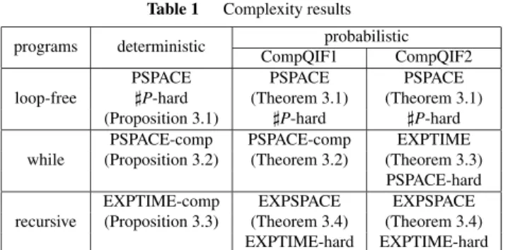
When we discuss lower-bounds, we consider the cor- responding decision problem by adding a candidate answer of the original problem as a part of an input. The results on the complexity of CompQIF1 and CompQIF2 are sum- marized in Table 1. As mentioned above, if a program is deterministic, QIF₁=QIF₂.

Recursive Markov chain (abbreviated as RMC) is de- fined in[13]by assigning a probability to each transition in

Table 1 Complexity results programs deterministic probabilistic

CompQIF1 CompQIF2

loop-free

PSPACE PSPACE PSPACE

P-hard (Theorem 3.1) (Theorem 3.1) (Proposition 3.1) P-hard P-hard while

PSPACE-comp PSPACE-comp EXPTIME

(Proposition 3.2) (Theorem 3.2) (Theorem 3.3) PSPACE-hard recursive

EXPTIME-comp EXPSPACE EXPSPACE

(Proposition 3.3) (Theorem 3.4) (Theorem 3.4) EXPTIME-hard EXPTIME-hard

recursive state machine (abbreviated as RSM)[1]. Proba- bilistic recursive program in this paper is similar to RMC except that there is no program variable in RMC. If we translate a recursive program into an RMC, the number of states of the RMC may become exponential to the number of Boolean variables in the recursive program. In the same sense, deterministic recursive program corresponds to RSM, or equivalently, pushdown systems (PDS) as mentioned and used in[9]. Also, probabilistic while program corresponds to Markov chain. We will review the definition of RMC in Sect. 3.6.1.

3.3 Deterministic Case

We first show lower bounds for deterministic loop-free, while and recursive programs. For deterministic recursive programs, we give EXPTIME upper bound as a corollary of Theorem 3.4.

Proposition 3.1: CompQIF1(=CompQIF2) isP-hard for deterministic loop-free programs even if the input values are uniformly distributed.

(Proof) We show thatSAT can be reduced to CompQIF1 where the input values are uniformly distributed. It is nec- essary and sufficient for CompQIF1 to compute the number of inputs ssuch that p(s|o) > 0 because

p(s|o)>0p(s) =

|{s ∈ S | p(s|o) > 0}|/|S|. For a given propositional logic formulaφwith Boolean variablesS, we just construct a pro- gramPwith input variablesS and an output variableOsuch that the value ofφforS is stored toO. Then, the result of CompQIF1 withPando=coincides with the number of

models ofφ.

Proposition 3.2: CompQIF1(= CompQIF2) is PSPACE- hard for deterministic while programs.

(Proof) The proposition can be shown in the same way as the proof of PSPACE-hardness of the non-interference problem for deterministic while programs by a reduction from quan- tified Boolean formula (QBF) validity problem given in[9]

as follows. For a given QBF ϕ, we construct a determin- istic while programPhaving one output variable such that Pis non-interferent if and only ifϕis valid as in the proof of Proposition 19 of[9]. The deterministic program is non- interferent if and only if the output of the program is always , i.e.,p()=1. Thus, we can decide ifφis valid by check- ing whether p()=1 or not for the deterministic program,

the output value, and the probability 1.

Proposition 3.3: CompQIF1(=CompQIF2) is EXPTIME- complete for deterministic recursive programs.

(Proof) EXPTIME upper bound can be shown by translat- ing a given program to a pushdown system (PDS). Assume we are given a deterministic recursive program P and an output valueo∈ O. We apply toPthe translation to a recur- sive Markov chain (RMC)Ain the proof of Theorem 3.4.

The size of Ais exponential to the size of P. Because P is deterministic, A is also deterministic; Ais just a recur- sive state machine (RSM) or equivalently, a PDS. It is well- known[8]that the pre-image of a configurationcof a PDS Apre_A(c)={c|cis reachable tocinA}can be computed in polynomial time by so-called P-automaton construction.

Hence, by specifying configurations outputtingo as c, we can compute pre_P(o)=pre_A(c) in exponential time.

The lower bound can be shown in the same way as the EXPTIME-hardness proof of the non-interference problem for deterministic recursive programs by a reduction from the membership problem for polynomial space-bounded alter- nating Turing machines (ATM) given in the proof of Theo- rem 7 of[9]. From a given polynomial space-bounded ATM M and an input wordwtoM, we construct a deterministic recursive programPhaving one output variable such thatP is non-interferent if and only ifMacceptswas in[9]. As in the proof of Proposition 3.2, we can reduce to CompQIF1 instead of reducing to the non-interference problem.

3.4 Loop-Free Programs

We show upper bounds for loop-free programs. For CompQIF2, the basic idea is similar to the one in[9], but we have to compute the conditional probabilityp(o|s). For CompQIF1,P^NPupper bound can be obtained by a similar result on model counting if the input values are uniformly distributed.

Theorem 3.1: CompQIF1 and CompQIF2 are solvable in PSPACE for probabilistic loop-free programs. CompQIF1 is solvable inP^NP if the input values are uniformly dis- tributed.

(Proof) We first show that CompQIF2 is solvable in PSPACE for probabilistic loop-free programs. If a program is loop-free, we can computep(o|s) for everysin the same way as in[9], multiply it by p(s) and sum up in PSPACE.

Note that in[9], it is assumed that a program is determin- istic and input values are uniformly distributed, and hence it suffices to count the input valuesssuch thatp(o|s) =1, which can be done inP^CH3. In contrast, we have to compute the sum of the probabilities ofp(s)p(o|s) for alls∈S. We can easily see that CompQIF1 is solvable in PSPACE for probabilistic loop-free programs in almost the same way as CompQIF2. Instead of summing upp(s)p(o|s) for alls∈S, we just have to sum upp(s) for alls∈Ssuch thatp(o|s)>0 (if and only ifp(s|o)>0).

Next, we show that CompQIF1 is solvable in P^NP

if the input values are uniformly distributed. As stated in the proof of Proposition 3.1, in this case, CompQIF1 can be solved by computing the number of inputs s such that p(s|o) > 0. Deciding p(s|o) > 0 for a given probabilis- tic loop-free programPcan be reduced to the satisfiability problem of a propositional logic formula. Note that for any probabilistic choice like X ← c1 r[]₁₋r c2 with 0 <r < 1, we just have to treat it as a non-deterministic choice like X =c1or X =c2 because all we need to know is whether p(s|o)>0. We construct fromPa formulaφwith Boolean variable corresponding to input and output variables of P and intermediate variables. Here, we abuse the symbolsS andO, which are used for the variables of P, also as the Boolean variables corresponding to them, respectively. The formula φis constructed such that φ∧S = s∧O = o is satisfiable if and only if p(s|o)¿ 0 forsando. Thus, the number of inputs s such that p(s|o) > 0 is the number of truth assignments forS such thatφ∧O =o is satisfiable, i.e., the number of projected models on S. This counting can be done inP^NPbecause projected model counting is in

P^NP[3].

3.5 While Programs

We show upper bounds for while programs. For CompQIF1, we reduce the problem to the reachability problem of a graph representing the state reachability relation. An up- per bound for CompQIF2 will be obtained as a corollary of Theorem 3.4.

Theorem 3.2: CompQIF1 is PSPACE-complete for proba- bilistic while programs.

(Proof) It suffices to show that QIF1is solvable in PSPACE for probabilistic while programs. QIF1 for probabilistic while programs is reduced to the reachability problem of graphs that represents the reachability among states of P.

We construct a directed graphGfrom a given programPas follows. Each node (l, σ) onG uniquely corresponds to a locationlonPand an assignmentσfor all variables inP.

An edge from (l, σ) to (l, σ) represents that if the program is running atlwithσthen, with probability greater than 0, it can transit tolwithσby executing the command atl. De- ciding the reachability from a node to another node can be done in nondeterministic log space of the size of the graph.

The size of the graph is exponential to the size ofPdue to exponentially many assignments for variables. We see that p(s|o) > 0 if and only if there are two nodes (ls, σs) and (lo, ρo) such thatlsis the initial location,lois an end loca- tion,σs(S) =s,σo(O) =o, and (lo, ρo) is reachable from (ls, σs) inG. Thus, p(s|o) >0 can be decided in PSPACE, and also

p(s|o)>0p(s) can be computed in PSPACE.

Theorem 3.3: CompQIF2 is solvable in EXPTIME for probabilistic while programs.

(We postpone the proof until we show the result on recursive

programs.)

3.6 Recursive Programs

As noticed in the end of Sect. 3.1, we will use recursive Markov chain (RMC) to give upper bounds of the complex- ity of CompQIF1 and CompQIF2 for recursive programs be- cause RMC has both probability and recursion and the com- plexity of the reachability probability problem for RMC was already investigated in[13].

3.6.1 Recursive Markov Chains

A recursive Markov chain (RMC)[13] is a tuple A = (A1, . . . ,Ak) where each Ai = (Ni,Bi,Yi,Eni,E xi, δi) (1 ≤ i ≤ k) is acomponent graph(or simply, component) con- sisting of:

• a finite setNiofnodes,

• a setEni⊆Niofentry nodes, and a setE xi⊆Niofexit nodes,

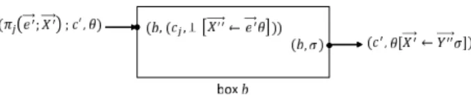
• a setBi ofboxes, and a mappingYi : Bi → {1, . . . ,k} from boxes to (the indices of) components. To each box b∈Bi, a set ofcall sites Callb={(b,en)|en∈EnYi(b)} and a set ofreturn sites Retb ={(b,ex) |ex ∈ E xY_i(b)} are associated.

• δi is a finite set of transitions of the form (u,pu,v, v) where

– the sourceuis either a non-exit nodeu ∈ Ni\E xi

or a return site.

– the destination v is either a non-entry node v ∈ Ni\Enior a call site.

– pu,v∈Qis a rational number between 0 and 1 rep- resenting the transition probability fromutov. We require for each sourceu,

{v|(u,p_u,v,v)∈δi}pu,v=1.

We writeu→^pu,vvinstead of (u,pu,v, v) for readabil- ity. Also we abbreviateu→¹ vasu→v.

Intuitively, a boxbwithYi(b) = jdenotes an invocation of component j from componenti. There may be more than one entry node and exit node in a component. A call site (b,en) specifies the entry node from which the execution starts when called from the boxb. A return site has a similar role to specify the exit node.

Let Qi = Ni ∪

b∈B_i(Callb∪Retb), which is called the set of locations of Ai. We also let N =

1≤i≤kNi, B =

1≤i≤kBi,Y =

1≤i≤kYi where Y : B → {1, . . . ,k}, δ=

1≤i≤kδiandQ=

1≤i≤kQi.

The probability pu,vof a transitionu ^p→^u,v vis a rational number represented by a pair of non-negative integers, the numerator and denominator. The size of pu,vis the sum of the numbers of bits of these two integers, which is called the bit complexityof pu,v.

The semantics of an RMCAis given by the global (infi- nite state) Markov chainMA =(V,Δ) induced fromAwhere V =B^∗×Qis the set of global states andΔis the smallest set of transitions satisfying the following conditions:

(1) For everyu∈Q, (ε,u)∈Vwhereεis the empty string.

(2) If (α,u) ∈ V andu →^pu,v v ∈ δ, then (α, v) ∈ V and (α,u)^p→^u,v(α, v)∈Δ.

(3) If (α,(b,en))∈V with (b,en)∈Callb, then (αb,en)∈ Vand (α,(b,en))→(αb,en)∈Δ.

(4) If (αb,ex)∈Vwith (b,ex)∈Retb, then (α,(b,ex))∈V and (αb,ex)→(α,(b,ex))∈Δ.

Intuitively, (α,u) is the global state whereuis a current lo- cation and αis a pushdown stack, which is a sequence of box names where the right-end is the stack top. (2) defines a transition within a component. (3) defines a procedure call from a call site (b,en); the box namebis pushed to the cur- rent stackαand the location is changed toen. (4) defines a return from a procedure; the box namebat the stack top is popped and the location becomes the return site (b,ex).

For a locationu∈Qiand an exit nodeex∈E xiin the same component Ai, letq^∗_(u,ex)denote the probability of reaching (ε,ex) starting from (ε,u)^†. Also, letq^∗_u =

ex∈E x_iq^∗_(u,ex). The reachability probability problem for RMCs is the one to computeq^∗_(u,ex)within jbits of precision for a given RMC A, a locationuand an exit nodeexin the same component ofAand a natural numberjin unary.

The following property is shown in[13].

Proposition 3.4: The reachability probability problem for RMCs can be solved in PSPACE. Actually, q^∗_(u,ex) can be computed for every pair of u and ex simultaneously in PSPACE by calculating the least fixpoint of the nonlinear polynomial equations induced from a given RMC.

3.6.2 Results

Theorem 3.4: CompQIF1 and CompQIF2 are solvable in EXPSPACE for probabilistic recursive programs.

(Proof) We will prove the theorem by translating a given programPinto a recursive Markov chain (RMC) whose size is exponential to the size ofP. By Proposition 3.4, we obtain EXPSPACE upper bound. Because an RMC has no program variable, we expand Boolean variables in P to all (reach- able) truth-value assignments to them. A while command is translated into two transitions; one for exit and the other for while-body. A procedure call is translated into a box and transitions connecting to/from the box. For the other com- mands, the translation is straightforward.

LetP=(π1, . . . , πk) be a given program. For 1≤i≤k, letVal(πi) be the set of truth value assignments toVar(πi).

We will use the same notationVal(e) andVal(c) for an ex- pressioneand a commandc. For an expressioneand an assignmentθ∈Val(e), we writeeθto denote the truth value obtained by evaluating eunder the assignment θ. For an assignmentθand a truth valuec, letθ[X←c] denote the as- signment identical toθexceptθ[X←c](X)=c. We use the

†Though we usually want to knowq^∗_(en,ex)for an entry nodeen, the reachability probability is defined in a slightly more general way.