Numerical and Experimental Studies on Dynamic Load Testing of Open‑ended Pipe Piles and its Applications
著者 ファン タ レ
著者別表示 Phan Ta Le journal or
publication title
博士論文要旨Abstract 学位授与番号 13301甲第3962号
学位名 博士(工学)
学位授与年月日 2013‑09‑26
URL http://hdl.handle.net/2297/37361
Creative Commons : 表示 ‑ 非営利 ‑ 改変禁止 http://creativecommons.org/licenses/by‑nc‑nd/3.0/deed.ja
Dissertation abstract
Numerical and Experimental Studies on
Dynamic Load Testing of Open-ended Pipe Piles and its Applications
開端杭の動的載荷試験に関する解析的・実験的研究とその適用
Graduate School of
Natural Science and Technology Kanazawa University
Division of Environmental Science and Engineering Course: Environment Creation
School registration No.: 1023142420
Name: Phan Ta Le
Chief advisor: Matsumoto Tatsunori
1
Abstract
Dynamic load test is one of the popular test methods to determine the pile performance. At present, Smith’s method, characteristic solution and a finite differential scheme have been used for dynamic analysis of the one-dimensional stress wave propagation in a pile. However, they still have limitation because the pile response and soil resistance are not fully coupled at a time step. Therefore, a matrix form calculation procedure of the one-dimensional stress wave theory is proposed in this thesis to improve the above shortcomings. In the proposed method, rational soil resistance models introduced by Randolph and Deeks (1992) are implemented. Effect of the wave propagation in the soil plug is modelled and taken into account. Furthermore, nonlinearity of soil stiffness and radiation damping are considered. The proposed method can also be used for the analysis of static loading condition. From numerical analyses, the proposed method showed higher accuracy compared to the Smith method and shorter calculation time compared to the rigorous continuum method FLAC3D. The proposed method well predicted the static response of small-scale model test as well as full-scale tests. Finally, the proposed method reasonably esti- mate static cone resistance of the dynamic cone penetration tests with dynamic measurement.
1. Background, motivation and objectives
At present, the two common pile load test methods are static load tests (SLTs) and dynamic load tests (DLTs). SLTs are considered the most reliable methods for determining the pile perfor- mance; however, they are costly and time-consuming. Therefore, about 1 to 2 % of working piles are selected for testing, resulting in a low reliability of the whole foundation solution. Meanwhile, DLTs which are low cost, short test period and very effective in offshore conditions. With the similar budget for testing, we can carry out up to 10 or 20% of the working piles, resulting in a high reliability of the whole foundation solution. Such high reliability would help us reduce factors of safety or cut down the cost of the whole project without reduction of safety of founda- tion solution. Therefore, research on dynamic analysis of DLTs is essential to seek for an efficient foundation solution to the structure.
In terms of dynamic analysis, there are several computer programs developed such as CAPWAP (Rausche el al. 1972, Goble et al 1976, 1979), TNOWAVE (Middendorp et al. 1986), KWAVE (Matsumoto et al. 1991), KWAVEFD (Wakasaki et al. 2004), TEPWAP (Paikowsky et al. 1982, 1990), PWAP (Paikowsky et al. 2008). However, they still have limitations concerning numerical method and soil resistance model itself. In the conventional analytical methods for the one-dimensional wave propagation problem, pile response and soil resistance are not fully coupled at a time step. Nonlinearity of soil stiffness and radiation damping are not considered.
Hence, a proposed numerical method based on the one-dimensional stress-wave theory using a matrix form and the modified rational soil models has been developed to improve the current pile dynamic analysis. The proposed method was then verified through numerical analyses and small- scale model tests. After that, the proposed method was used to analyses full-scale tests. Finally, the proposed method was used to identify the soil resistance acting on driving rod and cone tip of a dynamic cone penetration test with dynamic measurement.
2. Development of a numerical method for analysing wave propagation in an open-ended pipe pile
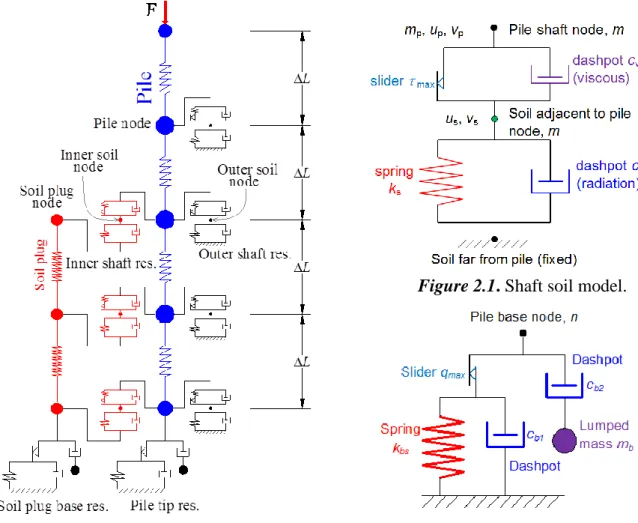
2.1. Numerical modelling
The numerical model for analysing the stress wave propagation in an open-ended pipe pile is shown in Fig. 2.1. In this model, the pile and the soil plug are modelled as a series of massless linear springs with discrete masses at the nodes. Outer frictional forces acting on the pile nodes as well as inner frictional forces acting between the soil plug nodes and the pile nodes are consid- ered. In the proposed numerical model, the soil reaction on the pile annulus and the soil reaction
2
beneath the soil plug are separately considered. The rational soil models proposed by Randolph and Deeks (1992) are implemented for both outer and inner soil resistances.
Figure 2.1. Shaft soil model.
Figure 2.2. Pile – soil system. Figure 2.3. Base soil model.
In the proposed method, non-linearity of the soil stiffness and radiation damping were im- plemented using empirical relation introduced by Chow (1986). Difference values of the maximum shear resistances when the pile moves downward and upward were also considered.
Plastic slider in the rational soil model was replaced by a slider connected to an interface spring in order to calculate the soil response at the same calculation time step with the pile response.
2.2. Formulation of calculations
Motion of the pile-soil system can be expressed by the well-known matrix form as follows:
K w
C w
M
w F (2.1) in which [K], [C] and [M] are the global stiffness, damping, and mass matrices, respectively. w , w , w and F are the displacement, velocity, acceleration and the applied force vectors, respectively.
Using the Newmark’s method, the incremental form of Eq. (21) is rewritten as:
2
2
t t
t t t
C M
K w
t t
0
1 1
2
F t t t K t w t C t Mtt w t
1 1
2 1
2 2 t 2 t t
t C M w
(2.2)
3
The coefficient terms of the matrix in the left hand side of the Eq. (2.2) are known. There- fore, the increment of the displacement vector, {w}t+t, for the pile, soil plug, outer soil, and inner soil can be solved readily. If the values of [C], [M] and viscous parameter of the rational soil model, are set to be zero, the above approach can be applied to a fully static problem.
2.3. Verification of the proposed method
In order to verify the proposed numerical method, a solid pile without soil resistance and an open-ended pile with soil resistance were analysed.
In the former analysis, the pile having a length, L, of 10 m was divided into 50 elements subjected to a triangle force with loading duration, tL, of 1 ms. Time step was set at different values, from 0.1 to 4 times critical time step, tcri, which is defined as a square roof of a half of a ratio of element pile length, L, to wave speed, c. When time steps were greater than 2tcri, solution could not be obtained. The calculation results using t = 0.5t cri gave the solutions which were the closest to the theoretical values in the figures. The calculation results using t = 0.1t cri were almost equal to those using t = 0.5t cri. Hence, t = 0.5t cri can be used in dynamic analysis; however, in case of nonlinear analysis, calculation time step should be selected to be much smaller than 0.5t cri in order to achieve an acceptable accuracy with reasonable calculation time.
In the later analysis, the open-ended pipe pile having a length, L, of 21 m in a uniform ground subjected by a sinusoidal impact loads with a peak value of 2500 kN and loading duration of 100 ms was analysed. The pile was divided into 42 elements. The calculation time step was set at 0.02 ms, about one third of critical time step. For the purpose of comparison, similar pile and soil condition were used in three methods. Note that the Smith and proposed method are simpli- fied methods based on the one-dimensional stress-wave theory using the rational soil models while FLAC3D is a three-dimensional explicit finite difference program.
For this analysis, the computational time in FLAC3D was more than 30 minutes while only a few second was taken in the proposed and Smith methods. The pile head displacements ob- tained from the proposed method well agree with those from the FLAC3D, while the Smith method underestimates the pile displacements obtained from the FLACcalculation (see Fig. 2.4).
Figure 2.4. Pile head displacements obtained from the three methods.
2.4. Conclusion on numerical studies
The following conclusions and findings were drawn from the numerical analyses:
(1) The results obtained from the proposed method are comparable with those obtained from the rigorous continuum method, the FLAC3D.
(2) The proposed method has a fast computation time when compared to the rigorous method.
0 20 40 60 80 100 120 140 160
0.0 10.0 20.0 30.0 40.0 50.0 60.0
Proposed method FLAC3D
Smith's method Pile head disp.,w h (mm)
Time, t (ms)
4
Although the validity of the proposed method was examined through numerical analysis, it is needed to verify the proposed method through experiments and field tests.
3. Validation of the proposed method through laboratory test 3.1. Test description
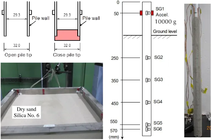
Two series of static and dynamic load tests of an open-ended pipe pile and a close-ended pipe pile were carried out in the model ground of dry sand, Silica No. 6, as shown in Fig. 3.1 to validate the proposed numerical method. The piles have a length of 600 mm and an outer diame- ter of 32 mm, and instrumented by 24 strain gauges at 6 levels, from SG1 to SG6. At each level, the strain gauges were attached symmetrically through the pile axis. Each location has two gauges to measure the vertical and horizontal strains. At the SG1 level, two accelerometers having a range of 10,000g were mounted next to the strain gauges on opposite sides.
Figure 3.1. Model piles and ground
3.2. Test procedure
For each pile, a series of pile load tests were carried out in four stages including (1) penetration test, (2) the first static load test (SLT1), (3) dynamic load test and (4) finally the second static load test (SLT2). In the case of the OP, the soil plug height was measured after each stage to investigate the plugging mode of the pile. In the case of the CP, an additional compression and tension tests were carried out to evaluate the difference in the outer shaft resistance between them.
3.3. Results of the close-ended pipe pile
A total of 5 blows were conducted from various falling heights with the small and big hammers.
The results of the wave matching analysis (WMA) of the last blow are presented because SLT2 was carried out right after this blow. The pile axial forces obtained from the measured strains at SG3, SG4 and SG5 were used as targets in the wave matching analysis.
Dry sand Silica No. 6
5
In WMA, the model ground was divided into 5 layers while the pile was divided into 55 el- ements. Calculation time step was set at 0.5s, a half of critical time step, tcri = L/(2c) = 1 s.
The measured pile axial force at SG1 in the last blow was used as the input head force. In the first WMA, a good matching was not obtained. The soil properties were then changed until a good matching between the calculated and the measured responses was achieved.
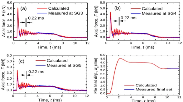
The results of the final WMA of the calculated and measured axial forces at SG3, SG4 and SG5 are shown in Fig. 3.3. At each level, the calculated axial forces were in close agreement with the measured forces. In the calculated results, oscillation with a period of 0.22 ms corresponds to the return travelling time, 2L/c, of the stress wave in the pile was found, indicating that the proposed numerical method is capable of calculating the wave propagation in a pile. Oscillation with a period of 0.22 ms is not seen in the measured forces. A possible reason for this might be due to the low frequency response of the amplifier used for the strain measurement.
Furthermore, a reasonable agreement in the final settlements between the calculated and the measured values was obtained as indicated in Fig. 3.3d.
The soil properties identified from the final WMA were then used to calculate the static load-displacement curve and compared with the static load test results as shown in Fig. 3.4. A reasonable agreement between the derived and the measured results was obtained.
Figure 3.2. Results of the final WMA of the CP for the axial forces and displacement.
(a) Force at SG3. (b) Force at SG4. (c) Force at SG5. (d) Pile head displacement.
Sensitivity of the analysed results due to variation of shear moduli and soil resistances were also investigated. The analysed results showed that the shear modulus has a lower sensitivity to pile response compared to the soil resistances. The soil resistance distribution could be estimated with an acceptable accuracy within a variation of 5 % if the differences between calculated and measured values of the peak upward travelling force and final pile head displacement in WMA are in range of 20 % and 5 %, respectively. Similar criteria could be used in WMA to obtain the distribution of shear modulus with an accuracy of 20 %. If measurements of elastic shear wave velocities of the ground are available we could improve the accuracy of the soil properties identified from WMA.
Influence of boundary of the soil box on the pile response was also examined. The return travelling time for the shear wave in the ground between the pile shaft and the side wall is 12.6 ms (= 2ds/cs = 0.0126 s) while the driving event terminates at about 9.0 ms after the impact, as shown in Fig. 3.2. Hence, it can be said that the side wall has no influence on the pile behaviour
0 2 4 6 8 10 12
0.0 1.0 2.0 3.0 4.0 5.0 6.0
0.22 ms
(a) Calculated
Measured at SG3
Axial force,F (kN)
Time, t (ms)
0 2 4 6 8 10 12
0.0 1.0 2.0 3.0 4.0 5.0 6.0
0.22 ms (b)
Time, t (ms)
Axial force,F (kN)
Calculated Measured at SG4
0 2 4 6 8 10 12
0.0 1.0 2.0 3.0 4.0 5.0 6.0
0.22 ms (c)
Time, t (ms)
Axial force,F (kN)
Calculated Measured at SG5
0 2 4 6 8 10 12
0.0 0.5 1.0 1.5 2.0 2.5 3.0 3.5 4.0 4.5 5.0
Calculated Measured final set
Time, t (ms)
Pile head disp., w h (mm)
6
during the pile driving test. Meanwhile, the reflected wave from the bottom of the soil container can reach the pile before the end of driving; however, this influence was not clearly seen from the measured axial force as shown in these figures.
3.4. Results of the open-ended pipe pile
Based on the experimental results, plugging mode of the open-ended pipe pile was found differ- ently between each test. In penetration test and dynamic load test, partially plugging mode were occurred while only perfectly plugging mode was found in both the SLT1 and SLT2.
WMA procedure was also conducted for the OP to identify the soil properties. The static load-displacement curve was then calculated using the soil properties identified from the final WMA are shown in Fig. 3.5, compared with the SLT results. The agreement between the derived and the measured values are seen in the figure.
Perfect plugging mode of an open-ended pipe pile under static loading condition and par- tially plugging mode under dynamic loading can be simulated using the proposed method.
Figure 3.3. Derived and measured static load- displacement curves of the CP.
Figure 3.4. Derived and measured static load- displacement curves of the OP.
3.5. Conclusions on experimental studies
The proposed method has the potential to estimate static responses of open-ended pipe piles and close-ended piles with a reasonable accuracy. Yield load and ultimate capacity (defined as a load at a settlement of 0.1D) of the OP was smaller than those of the CP.
The proposed method has been verified using numerical analysis in Section 2.3, and small scale experiments in this section. Hence, the proposed method will be used to analyse the full- scale test in the following section for further verification.
4. Analysis of a case study in Viet Nam using the proposed method 4.1. Introduction
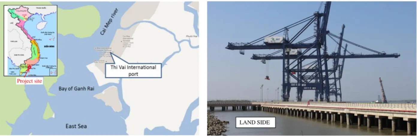
A berth structure, 600 m long and 60 m wide, has been completed at Thi Vai International Port located on the bank of the Cai Mep River in Viet Nam in 2013 as shown in Fig 4.1. The berth structure is supported by more than one thousand piles including 885 driven spun concrete piles (SCP) and 156 driven steel pipe piles (SPP). Test piling was conducted in 2011 to obtain design parameters and to seek for driving control and quality assessment methods for constructed piles.
Four test piles were carried out prior to construction of working piles. Two of them were spun concrete piles designated as TSC1 (D=700 mm) and TSC2 (D=800 mm), and the other two piles were open-ended steel pipe piles designated as TSP1 (D=1000 mm) and TSP2 (D=900 mm).
All the test piles were driven into the ground using a diesel hammer having a ram mass of 10 tons.
4.0 3.5 3.0 2.5 2.0 1.5 1.0 0.5
0.00.0 0.2 0.4 0.6 0.8 1.0 1.2
SLT from WMA Head force, Fh (kN)
Pile head displacement,wh (mm)
4.0 3.5 3.0 2.5 2.0 1.5 1.0 0.5
0.00.0 0.2 0.4 0.6 0.8 1.0 1.2
Soil plug base resist.
Tip resist.
SLT From WMA
Total resist. Shaft resist.
Pile tip resist. SP base resist.
Head force or Resistance (kN)
Pile head displacement,wh (mm)
7
Dynamic load tests (DLTs) of the TSC1 and TSP1 were carried out at the end of driving work (EOD tests) and beginning of re-striking tests (BOR tests) were conducted after curing periods of 7 days for the TSC1 and 34 days for the TSP1. Static load tests (SLTs) were carried out 10 days later for the TSC1 and 14 days later for the TSP1. SLT was also carried out for the TSC2 and TSP2 after the rest periods of 17 days and 27 days from the completion of the driving work.
Figure 4.1. Location of the site and photo of the berth area after completion in 2013 In this part, wave matching analysis (WMA) of the DLTs at initial driving and re-striking of the TSC1 and TSP1 are conducted using a numerical approach developed by the authors to identify the soil parameters which are used for calculating the static load-displacement relations.
After that, static load-displacement relations of the TSC2 and TSP2 are predicted using the soil parameters identified from the WMA of the TSC1 and TSP1 in order to evaluate the applicability of the proposed WMA to quality assessment of the constructed piles.
4.2. Site and test description
The ground consists of three soil layers with different thickness from pile to pile. Typically, very soft clay exists from the seabed to depths of 6 m to 20 m. Below this top layer, a clayey sand of about 25 m thick with loose state at the top to medium dense state at the bottom exists, being underlain by hard silt clay that could be regarded as a bearing stratum. All the test piles were driven into the bearing stratum of the hard silt clay, resulting in the different embedment pile lengths. Then, the test piles were cut to the cut-off level for the testing work. The final pile length were 54 m, 48.7 m, 60 m and 49.9 m for TSC1, TSC2, TSP1 and TSP2, respectively.
DLTs were carried out at the end of driving (EOD) and at the beginning of re-striking (BOR) using a hammer mass of 10 ton. Two strain gauges and two accelerometers were attached near the pile head to measure strains and accelerations during driving. The settlement per blow of the pile head was also manually measured at the end of each blow. SLT was carried out after a given rest period from the BOR test to obtain the static load-displacement relation. In SLT, reaction force was created by 8 steel pipe piles having a diameter of 700 mm and a length of about 40 m. The static load test was carried out in two cycles with 21 loading and unloading steps 4.3. Wave matching analysis and test results of the TSC1
Modelling of the test ground at the test site of the test pile TSC1 is shown in Fig. 4.2. The ground was divided into 5 sub-layers and the test pile, TSC1, having a length of 54 m was divided into 54 elements in the WMA. Calculation time step was set at 0.01ms, one tenth of critical time step,
tcri = L/(2c) = 0.1 ms. Distribution of shear moduli and shear resistances with depth were estimated based on the distribution of the SPT N-values.
The impact head force, F(0,t), was calculated from the measured force and measured veloc- ity based on the one-dimensional stress-wave theory. Pile axial force, downward and upward traveling forces, velocities and displacements obtained from the measured dynamic signals at the strain gauge level were used as targets in WMA.
Project site
LAND SIDE
8
Figure 4.2. Modelling of the test ground at the test pile TSC1.
In WMA with the first assumption of the soil properties, good matching was not obtained.
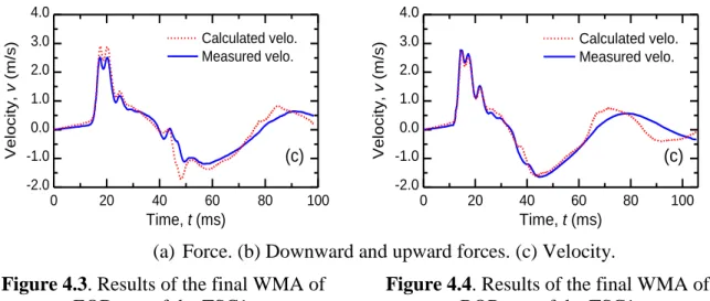
Then, the soil properties were changed until getting a good matching between the calculated and the measured responses. The results of the final WMA for both EOD and BOR tests are shown in Figs. 4.3 and 4.4, respectively.
As seen from the figures, the analysed results obtained from the final WMA are comparable with the measured values for both EOD and BOR tests. “Set-up” phenomenon is clearly found from the waveforms of the axial force and upward travelling force.
45 40 35 30 25 20 15 10 5 0
45 40 35 30 25 20 15 10 5
0 0 20 40 60
45 40 35 30 25 20 15 10 5
0 0 100 200
45 40 35 30 25 20 15 10 5
0 0 50 100 150
Depth from G.L. (m)
Soil profiles
TSC1
Hard silty clay Clayed
sand Soft clay
Interpolated Modelling
SPT N-value Shear modulus, G0, MPa
Shear resistance,
max, kPa
0 20 40 60 80 100
-1000 0 1000 2000 3000 4000 5000 6000
(a)
Calculated force Measured force
Axial force, F (kN)
Time, t (ms)
0 20 40 60 80 100
-1000 0 1000 2000 3000 4000 5000 6000
(a)
Calculated force Measured force
Axial force, F (kN)
Time, t (ms)
0 20 40 60 80 100
-2000 -1000 0 1000 2000 3000 4000 5000 6000
(b)
Calculated downforce Measured downforce Calculated upforce Measured upforce
Force, Fd andFu (kN)
Time, t (ms)
0 20 40 60 80 100
-2000 -1000 0 1000 2000 3000 4000 5000 6000
(b)
Calculated downforce Measured downforce Calculated upforce Measured upforce
Force, F d andF u (kN)
Time, t (ms)
9
(a) Force. (b) Downward and upward forces. (c) Velocity.
Figure 4.3. Results of the final WMA of EOD test of the TSC1.
Figure 4.4. Results of the final WMA of BOR test of the TSC1
Soil properties identified from the final WMA were used to calculate the static load- displacement curves. Figure 4.5 shows such curves derived from the EOD and BOR tests, com- pared with the static load test result in two cycles of loading process. As seen from the figure, the stiffness of the derived static response obtained from the BOR test is higher than that obtained from the EOD test, indicating the “set-up” phenomenon discussed previously. The derived static response obtained from the final WMA of the BOR test is comparable with the SLT, compared to that obtained from the EOD test. The three load-displacement curves in Fig. 4.5 clearly indicate the “set-up” phenomenon during the period from the EOD test via the BOR test to the SLT.
4.4. Wave matching analysis and test results of the TSP1
Similar to the TSC1, WMA was conducted for the TSP1, and the soil properties identified from the final WMA were also used to calculate the static response, and compared with the static load test result in two cycles of loading process as shown in Fig. 4.6. “Set-up” phenomenon is also found from this figure and the static response derived from the final WMA of the BOR test is comparable with the SLT result.
Figure 4.5. Comparison of the static load displacement curves of the TSC1.
Figure 4.6. Comparison of static load dis- placement curves of the TSP1.
If we compare the “set-up” phenomenon between two piles, we clearly seen that the degree of “set-up” phenomenon from EOD to BOR of the TSC1 are remarkable compared to those of the TSP1 although the rest period between EOD and BOR in the TSC1 (7 days) was shorter than that in the TSP1 (34 days). The different degrees of the "set-up" between the TSC1 and the TSP1 might be explained by different pile wall thicknesses which caused the different excess pore water pressure of the soil surrounding the pile during driving.
0 20 40 60 80 100
-2.0 -1.0 0.0 1.0 2.0 3.0 4.0
(c)
Calculated velo.
Measured velo.
Velocity, v (m/s)
Time, t (ms)
0 20 40 60 80 100
-2.0 -1.0 0.0 1.0 2.0 3.0 4.0
(c)
Calculated velo.
Measured velo.
Velocity, v (m/s)
Time, t (ms)
30.0 25.0 20.0 15.0 10.0 5.0
0.00 1000 2000 3000 4000
BOR EOD
SLT
SLT
from WMA_EOD from WMA_BOR Head force, F
h (kN)
Pile head displacement,wh (mm)
100.0 90.0 80.0 70.0 60.0 50.0 40.0 30.0 20.0 10.0
0.00 2000 4000 6000 8000
BOR
EOD SLT
SLT
from WMA_EOD from WMA_BOR Head force, F
h (kN)
Pile head displacement,w h (mm)
10
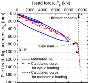
The TSP1 was reused as a working pile after the SLT with two cycles of loading processes.
Therefore, the pile TSP1 was further loaded until the pile reaches the ultimate bearing capacity to evaluate the influence of capacity caused by cyclic loading. This static response was compared with that obtained from analysis of the similar pile for a monotonic loading as shown in Fig. 4.7.
The author found that the yield load and the ultimate bearing capacity of the TSP1 after the two cycle of loading process are similar to those of the TSP1 subjected to only monotonic loading.
This means that cyclic loading has minor influence on the load-displacement curve at the pile head, if reduction of the shaft resistance due to cyclic loading does not occur.
Figure 4.7. Calculated load-displacement curves with and without cyclic loading, together with the result of SLT of the TSP1.
4.5. Prediction of static load-displacement curves for other test piles
The static responses of the TSC2 and TSP2 were predicted using the soil parameters identified from the final WMA of the TSC1 and TSP1, respectively. The predicted curves are then com- pared with the load-displacement relations obtained from the static load tests as shown in Fig. 4.8.
Figure 4.8. Comparison of the static curves of (a) The TSC2. (b) The TSP2
As seen from these two figures, the predicted curves are comparable with the measured ones. This means soil parameters identified from the WMA of the tested piles could be used to estimate the static responses of the other non-tested working piles in this construction site.
180.0 160.0 140.0 120.0 100.0 80.0 60.0 40.0 20.0
0.00 2000 4000 6000 8000 10000 Ultimate capacity
Yield load 0.1D
Measured SLT Calculated curve for cyclic loading Calculated curve for monotonic loading
Head force, Fh (kN)
Pile head displacement,w h (mm)
25.0 20.0 15.0 10.0 5.0
0.00 1000 2000 3000 4000 5000 6000
(a)
Measured SLT Predicted SLT Head force, Fh (kN)
Pile head displacement,wh (mm)
60.0 50.0 40.0 30.0 20.0 10.0
0.00 2000 4000 6000 8000
(b)
Measured SLT Predicted SLT Head force, Fh (kN)
Pile head displacement,wh (mm)
11 4.6. Conclusions on analysis of a case study
Based on the analysed results of the case study, the following findings and implications were drawn:
(1) The static load-displacement curves derived from the final WMAs of DLTs were com- parable with the results obtained from the SLTs.
(2) WMA using the proposed numerical approach can be used to predict the static load- displacement curves of the non-tested working piles based on the identified soil param- eters of the tested piles.
(3) The piles which have been subjected to cyclic loading have similar yield and ultimate capacities to those of the piles subjected to monotonic loading.
5. Application of the proposed wave matching procedure to DCPT and SPT 5.1. Test description
Twelve dynamic cone penetration tests (DCPTs) using various driving rods and a SPT in Fig. 5.1 were conducted for measuring impact energy transferred to the rods in Shiga prefecture in 2012.
Figure 5.1. DCPTs with dynamic measurements using various driving rods
In each test, two accelerometers and two vertical strain gauges were attached symmetrically near the rod head. The driving rod was first penetrated to the depth of about 5.5 to 6.0 m, and then connected to the instrumented rod and driven into the ground to measure the dynamic signals. For the first several blows, dynamic signals and settlement were measured for each blow called “initial blow”. After that, the driving rod was penetrated continuously by multiple blows (called “successive blow”) with penetration depth of 100 to 250 mm. Note that Test No. 1, Test No. 4 and several first blows of Test No. 6 used rubber cushion on the top of driving rod.
5.2. Results of measured driving energy for various types of DCPTs and SPT
Results of the energy efficiencies of the various DCPTs and the SPT are shown in Fig. 5.2. In can be clearly seen that the energy efficiencies mostly vary from 60 to 80 % in case of no cushion, and reduce about 20 % in case of using cushions (see Tests No. 1 and No.4). Distribution with depth of dynamic cone resistance, qdyn, calculated from energy conservation law was comparable with the static cone resistance, qt, obtained from cone penetration test (CPT). Note that qdyn
contains the static and dynamic components. Therefore, the higher values with depth of qdyn, compared to qt, are reasonable.
Moreover, different degree of “set-up” phenomenon was found between the “initial blows”
and the “successive blows”. This might be due to the difference in the rest period between them.
12 5.3. Wave matching analysis and test results
WMA of two blows of an example of DCPT with dynamic measurement (Test No. 12) were conducted, Blow 12.1 with cone tip level at depth of 5.8 m and Blow 12.2 at depth of 6.0 m. The cone tip resistance identified from WMA of Blows 12.1 and 12.2 were then compared to the static cone tip resistance obtained from CPT in Fig. 5.3. The figure indicates that the values identified from the final WMA of DCPT were comparable with that obtained from CPT.
Figure 5.2. Results of energy efficiency of various DCPTs with dynamic measurement
Figure 5.3. Comparison of static cone resistance from CPT and from WMA 5.4. Conclusions on application of the proposed WMA to DCPT
Advantages of DCPT and SPT with dynamic measurements were demonstrated in this study.
Proposed numerical method could be used to identify the static cone resistance. The energy efficiencies of various tests in this particular site vary from 40 % to 80 %. This suggests that DCPTs and SPT with dynamic measurement should be carried out in various soil conditions in order to obtain a possible range of energy efficiency for each test device.
6. Conclusions of the thesis
In this thesis, a proposed numerical method for analysing the one-dimensional propagation of stress-wave in an open-ended pipe pile was developed using a matrix form with Newmark’s method. The proposed numerical method used the rational soil resistance models with appropriate modification for improving the limitation of the conventional methods. First, the proposed method was verified through numerical analyses and small-scale model tests in laboratory. After that the proposed method was used to analyse a full-scale test in practice. Finally, the proposed method was employed to identify the soil resistance acting on the driving rod and cone tip of a DCPT with dynamic measurements. The following conclusions and findings were drawn from the limited analyses as follows:
(1) Higher accuracy of the proposed method was demonstrated compared to the conventional Smith’s method.
(2) Quickness in calculation compared to the rigorous continuum method, FLAC3D.
(3) The WMA using the proposed method has high potential to estimate static responses of very small and short piles in laboratory as well as very long and large piles in practice. The proposed method can also be used to identify the distribution with depth of static cone re- sistance of DCPTs and SPT with dynamic measurements.
(4) The proposed WMA procedure can be used as a practical alternative to the conventional static load test.
7.5 7.0 6.5 6.0 5.5
5.00 20 40 60 80 100
Test01 Test02 Test03 Test04 Test05 Test06 Test07 Test08 Test09 Test10 Test11 Test12 Driving energy efficiency, Eeff (%)
Depth from ground level,z (m)
7.5 7.0 6.5 6.0 5.5
5.00 2 4 6 8 10 12
Depth from ground level, z (m)
CPT WMA of Test 12 Static cone resistance, qt and qmax (MPa)