So we introduce two physical variables in our model, i.e. the space-efficient factor and the time-efficient factor. The former represents the factor which promotes

Abstract

We are often confused about the gap between the production theory and the real economy. That is attributed in part to the fact that many types of production functions have been imposed the unrealistic assumptions such as the homotheticity.

On the other hand, the economies of scale, especially with non-homotheticity, have been often disregarded although they are dominant phenomena in the real economy.

Many empirical studies, however, have verified that the economies of scale are in reality existent. Moreover, they have shown through using cross section data that the factor proportions are variable with the changes of productive scale even under constant relative prices. Those are derived from the differences of output-elasticities for each input. In addition, we can often find out negative elasticities of substitution among inputs in empirical studies. Behind these are the fact that qualitative factors in products have a significant role in the real economy. And then, we investigate what causes the economies of scale in actual productive activities. For this purpose, we set up the concepts of space and time as productive fields. Actual producer's behavior depends not only on economic variables (prices and quantities), but also on physical or engineering variables, which have relatively high degree of autonomy.

So we introduce two physical variables in our model, i.e. the space-efficient factor and the time-efficient factor. The former represents the factor which promotes

Skepticism to the Homotheticity, and Economies of Scale

― A Different Approach to

Analyzing the Real Economy ― Yoshiaki Araki

＊

Faculty of Economics, Fukuoka University, Fukuoka, Japan

−５ ３−

（ １ ）

technological efficiency by increasing in degree of production-intensity into space.

The latter represents the factor which promotes technological efficiency by increasing in degree of production-intensity into time. The specific variables corresponding to the two factors above differ with respect to each sector. For example, the specific variables corresponding to the space-efficient factor are weight, volume etc., and the ones corresponding to the time-efficient factor are velocity, turnover ratio etc.. In the productive fields of domestic freight transport, the weight and the velocity are the specific variables corresponding to the two factors above, respectively. Where the weight indicates the loading weight (tons) by each freight transport, and the velocity indicates the running distance per time required for each freight transport (kilometers). The term “scale" means productive capacity. Fundamentally, it is a function of two types of elementary factors above. And the differences of output- elasticities for each input (non-homotheticity) and economies of scale are basically generated from the difference of dimensions between output and inputs, through varying degree in production-intensity of each of the two factors above into space and time. Furthermore, the qualities of products make an important effect on producer's behavior for determining the degree of choice between the two factors above, as with economic variables. We will examine the above matters through analysis of the domestic freight transport industry.

1. Introduction

Haavelmo (1944) emphasized the importance of “the degree of autonomy”

in economic analysis. In fact, the difference of the degree of autonomy between the cost function and the production function in the production theory

1

It is a problem of recognition on real phenomena rather than a problem of pure logic on them. For instance, the weather (precipitation, temperature, etc.) has a direct influence on economic activities (especially, on agriculture). But the reverse is not true. We can recognize that there is a one-way relationship between them. Therefore we cannot forecast the weather from the outcome of economic activities (the change of relative prices etc.). However, the weather is irrelevant to an input variable of production function because we cannot control it.

−５ ４−

（ ２ ）

is an axiomatic truth. None the less, the dual theorem on them seems to be prevalent in recent theories. In most cases, it relies on the assumption that the production function is homothetic and quasi-concave. Therefore, the theory with the assumption above cannot consist with Adam Smith's theory on the division of labor and cannot necessarily account for familiar economic phenomena like M&A. We have received little explanation why unrealistic assumptions such as the homotheticity are imposed on it. One of the reasons to be considered is partially due to easiness of mathematical analysis.

Furthermore, the others would be to apply the Euler's theorem to the income distribution theory, and to find the equilibrium solution of the producer's behavior theory. Putting the easy-to-use approach before the matters in the real economy, however, could be thought to be similar to “Procrustean Bed".

We might be able to expect an alternative theory for research in accordance with the real economy in the near future.

2. Why don't the homotheticity come into existence in the real economy?

The homothetic function is a monotonic transformation of a linear homogeneous function. Therefore, the output-elasticities for all inputs are equal at any given point. If the production function is linearly homogeneous, all of them must equal to unity as a matter of course. In addition, the cost function can be expressed as the product of the two functions, one of output quantity and one of input prices. Many empirical studies, however, have provided conflicting evidence against the above theory. For example, Ozaki (1970) demonstrated the fact that the output-elasticities for inputs are different from each other under constant relative prices, especially ones for labor are Skepticism to the Homotheticity, and Economies of Scale（Araki） −５ ５−

（ ３ ）

smaller than unity. Then what makes these results arise from?

3. Basic relations generating the economies of scale

Chenery (1953) presented the paper on the engineering production function before. He pointed out that all inputs are categorized two different types.

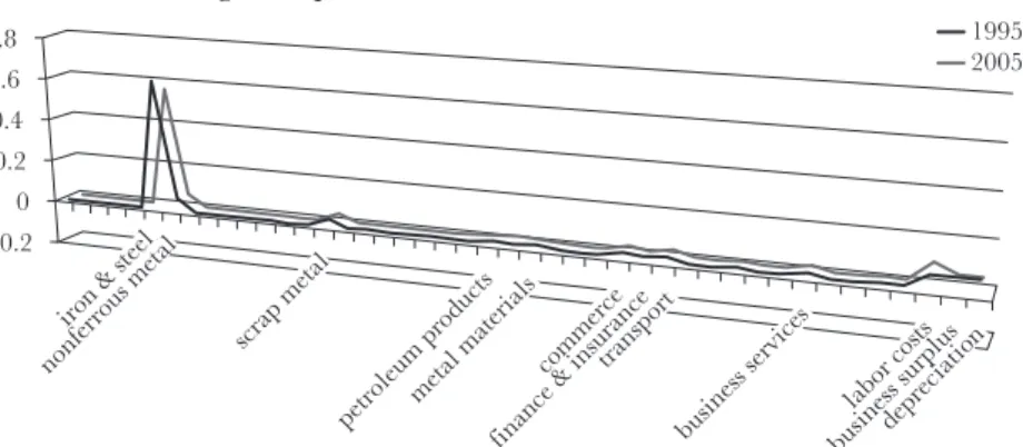
One are materials built into outputs, the other are “processing factors” (labor, capital goods, land and etc.). The former input coefficients are basically decided by design-specification, the latter ones have wider flexibility for the change of output quantities and of relative prices. In the sectors defined properly on engineering basis, the input coefficients of materials are relatively stable (See Fig.1〜Fig.4)

.

2

Actually, the input coefficients of materials vary slightly because there are more or less the product-mix and the change of yield rates. However, their variations are relatively small in comparison with the case of processing factors.

Fig. 1 Input coefficients of the crude steel sector 0.8

0.6 0.4 0.2 0 -0.2

1995 2005

iron & steel

nonferrous metal scrap metal

petroleum products metal materials commerce finance & insurance

transport

business services

labor costs depreciation business surplus (Source) The Input-Output tables with constant prices (published by the Ministry of Internal and

Communications in Japan)

All of input coefficients are in real terms (2005prices).

We calculated input coefficients of each sector aggregated on engineering basis.

−５ ６−

（ ４ ）

Fig. 2 The Change rates of input coefficients and relatve prices (2005/1995-1) in the crude steel sector

(Source) the same as Fig.1.

(change rates)＝(2005data)/(1995data)− 1

However, input coefficients less than 0.01 are omitted.

iron & steel nonferrous metal

scrap metal

petroleum products

belongings commerce transport services labor costs business surplus depreciation finance & insurance

0.8 0.6 0.4 0.2 0 -0.2 -0.4 -0.6

chang e r at es

sectors

relative prices input coefficients

Fig. 3 Input coefficients of the architecture (non-residence) sector 0.4

0.3 0.2 0.1 0

1995 2005

cement

machinery & parts furnishings iron & steel ceramics

chemical products

petroleum products

belongings commerce

finance & insurance transport

business services

labor costs business surplus depreciation (Source) the same as Fig.1

Skepticism to the Homotheticity, and Economies of Scale（Araki） −５ ７−

（ ５ ）

In fact, the input coefficients in more disaggregated sectors exhibit stronger technological complementarity among materials rather than substitutability among them. Therefore we can understand that the latter is largely caused by product-mix etc. in each sector. And the output quantity mainly depends on the cubic volumes of the vessels (or capital goods)and their processing velocities in space and time (three- dimensional or four-dimensional dependence). On the other hand, the input quantities of processing factors have considerable degree of dependence on the length or the area of the vessels (or capital goods)(one-dimensional or two-dimensional dependence) . Because of this, variations of the input coefficients for the processing factors are consequently due to the difference of dimensions between output and these factors in space and time, in addition to the product-quality and to the change of relative prices of them. Actually, we can often observe that the input Fig. 4 The Change rates of input coefficients and relatve prices (2005/1995-1) in the

architecture (non-residence) sector

(Source)the same as Fig.2

machinery & parts

furnishingiron & steelceramics

chemical products petroleum products

belongings commerce transport

business services labor costs business surplusdepreciation finance & insurance

0.8 0.6 0.4 0.2 0 -0.2 -0.4 -0.6

chang e r at es

sectors

relative prices input coefficients

−５ ８−

（ ６ ）

coefficients change inversely with expected direction against the variation of relative prices in many sectors (See Fig. 2 and Fig. 4)

. The fact-findings above are inconsistent with the homotheticity of the production function.

Therefore, we would like to explain the reason why the economies of scale with non-homotheticity are generated in the real economy, through introducing physical variables. For this purpose, we set up the concepts of time and space as production fields. If we can consider the production capacity as the flow of fluid per given time-span, the ratio of the volume and the velocity to the length of the line or the area in space and time can be divided into two types of elementary factors, namely, the space-efficient factor (S) and the time-efficient factor (T). The former represents the factor which promotes technological efficiency by increasing in degree of productive intensity in space, and the latter represents the factor which promotes technological efficiency by increasing in degree of productive intensity in time.

3

That means certain input coefficients increase in spite of the rise in their relative prices, and the similar often holds for the reverse case (the fall in their relative prices). For example, in the automobile sector, the input coefficient of plastics has an upward tendency in spite of the rise in its relative price after oil crisis. The reason is that weight reduction of the body should be necessary for improving fuel consumption (the quality of product). The elasticity of substitution is not always non-negative.

4

The way of our study is based on the principle of (fluid) dynamics. Providing a specific example of the construction sector, a rise in land prices regarded as horizontal space-costs should cause the conversion to high-rises (the substitution for vertical space). On the other hand, a rise in interest-rate regarded as a sort of time-costs should hasten the reduction of construction- period (the increase of construction-velocity).

Skepticism to the Homotheticity, and Economies of Scale（Araki） −５ ９−

（ ７ ）

Those are

S = S ( ׬ ߨ൫݂ሺ݈ሻ൯

݈݀

ʹߨ ׬ ݂ሺ݈ሻටͳ ൅ ቀ

ቁ

݈݀

൙ )

v

(1)

where the notations are as follows.

π: the circumference ratio, a & b : the limits of a solid revolution in space, l: the length of the line in space (variable).

and

ൌ ሺ׬ ߩ _஺ ࢜݀ܣȀ ׬ ܣԢሺ݈ሻ݈݀ _௔ ^௕ ሻ

v

(2)

where the notations are as follows.

A: the cross-section area of the fluid flow, ρ: the density of the fluid, v: the velocity vector.

A': the cross-section area of a solid revolution.

The first equation expresses the ratio of the volume of a solid revolution (for example, capital goods etc.) to its length or its area. This equation shows that the above ratio increases with making larger volume of a solid revolution because of the difference of the power numbers of function f(l) in the numerator and denominator (i.e. because of the difference of dimensions between output and inputs). For instance, we can provide a specific example of cubic volume of a blast furnace etc. On the other hand, the second equation expresses the mass flow of the fluid per the volume of a solid revolution. This equation shows that the ratio of the fluid flow to the area of a solid revolution increases with gaining in velocity. For instance, improvements of capital goods and changes of productive system (e.g. the division of labor, more generally, the division of productive processes) increase the velocity of productive activities.

−６ ０−

（ ８ ）

Provided the ratio of the volume and the velocity of the fluid flow to the length and the area of capital goods rises, the economies of scale should work particularly for the processing factors. The matters above, of course, have the limitations of the times on technology, cost and market size. The economies of scale, however, arise from the difference of dimensions between output and inputs fundamentally.

4. The mathematical model

Let us build the mathematical model based on the inquiry above.

The production function (based on engineering or physical relationship)

Q = f ( S , T ) (3)

where the notations are as follows.

Q: the production capacity S: the space-efficient factor T: the time-efficient factor The input functions

ܴ

= ȭ ( S , T, G ) ( i = 1, 2, ࣭࣭࣭, m ) (4)

ܯ

= ȯ ( S , T, G ) ( j = 1, 2, ࣭࣭࣭, n ) (5)

where the notations are as follows.

R

: the input quantity of i-th processing factor M

: the input quantity of j-th material factor

G: the factors which have little influence on the production capacity Skepticism to the Homotheticity, and Economies of Scale（Araki） −６ １−

（ ９ ）

but have a lot of influence on input quantities (e.g. the measures to ensure safety in productive activities, the prevention of environmental pollution and the frequency of cargo-transshipment in the transport industry etc.)

The cost equation ൌ ෍ ܲ

ܴ

൅

୫ ୧ୀଵ

෍ ܲ

ܯ

൅ܲ

ܵ

൅

୬ ୨ୀଵ

(6)

where the notaions are as follows.

P

: the price of i-th processing factor P

: the price of j-th material factor

P

: the opportunity cost per space of the product It represents a kind of quality of the product.

S

: the space size occupied by the product F: the fixed cost

The necessary condition for the cost minimization

ܥ

/ ܳ

= ܥ

/ ܳ

(7)

where the above suffixes represent partial derivatives of C and Q with respect to S and T

The sufficient condition for the cost minimization Bordered Hessian

ተተ

Ͳ ܳݏ ܳ

ܳݏ ቀܥݏݏ െ

ܳݏݏቁ ቀܥ

െ

ܳ

ቁ

ܳ

ቀܥ

െ

ொ௦

ܳ

ቁ ቀܥ

െ

ொ௦

ܳ

ቁ

ተተ ൏ 0 (8)

−６ ２−

（ １ ０ ）

5. The application of the specified model to the freight transport industry

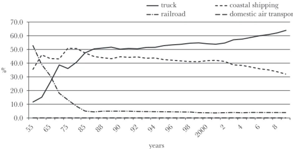
Let us show some fact-findings on the domestic freight transport industry in Japan before building the specified model. Most of domestic freight transportation volume calculated on a ton-kilometer basis are done by using truck, railroad and coastal shipping. First the share of transport by truck within the total domestic freight volume has increased, and the one by railroad has decreased during the past half century (see Fig. 5). Second the advantage of transport by truck is its high-speed performance, and the one by coastal shipping is its low-cost bulk shipment. Third the goods with short-haul and high-price per unit weight mainly depend on transport by truck, and the goods with long-haul and low-price per unit weight mainly depend on one by coastal shipping respectively (see Fig. 6).

Fig. 5 the transport-share transition by each traffic-means

(Source) The transport statistics of Ministry of Land, Infrastructure, Transport and Tourism in Japan.

55 55

55 65 65 65 75 75 75 85 85 85 88 88 88 90 90 90 92 92 92 94 94 94 96 96 96 98 98 98 2000 2000

2000 2 2 4 4 6 6 8 8

70.0 60.0 50.0 40.0 30.0 20.0 10.0 0.0

%

years truck railroad

coastal shipping domestic air transport Skepticism to the Homotheticity, and Economies of Scale（Araki） −６ ３−

（ １ １ ）

We will build the specified model based on some fact-findings above.

The (engineering or physical) production function specified with the Douglas form

ܳ

= ן

ܹ

ܸ

(9)

where the notations are as follows.

Q

: the volume of each transport (the freight ton-km by each transport) W: the batch of load (the weight of loading by each transport) V: the velocity of each vehicle (the running distance per time required

for each transport)

Q

, W and V represent proxy variables of Q, S and T, respectively.

The linear input functions

ܴ

= ܽ

+ ܽ

W + ܽ

V + ܽ

ܩҧ (i = 1,2,…,m) (10) ܯ

= ܾ

+ ܾ

W + ܾ

V + ܾ

ܩҧ (j = 1,2,…,n) (11) Fig. 6 The transport-share of each product by truck and by coastal shipping

(Source) the same as Fig.5

80%70%

60%50%

40%30%

20%10%

0%

g rain fr uit & v egit ables o ther f ar m... liv es toc k pr oducts aq uatic pr oducts w ood fire w ood & c har coal coal me talic miner als g ra vel & s tones non-me tallic... me tals me tal goods mac hines cement o ther cer amics pe tr oleum... chemicals chemical f er tilizer s dy e & paints paper & pulp fi b er s foods tuf fs dail y necessar ies rubber & w ood... specialized... no t classif iable truck coastal shipping

−６ ４−

（ １ ２ ）

where the notations are as follows.

R

: the input quantity of i-th processing factor M

: the input quantity of j-th material.

However, we can consider M_j as nothing in most service industries (including transport industry).

The cost equation ൌ ෍ ܲ

ܴ

൅

୫ ୧ୀଵ

ܲ

൅ (12)

where F is the fixed costs concerned with the service lines (the highway and delivery system, the railway-tracks and stations etc.)

The necessary condition of cost minimization ܥ

ܳ

൘ = ܥ

ܳ

൘ (13)

therefore

ሺܪ

൅ ܲ

ሻܹ

ן

ൗ = ܪ

ܸ ן

ൗ (14)

where ܪ

ൌ ෍ ܲ

ܽ

ǡ

୫ ୧ୀଵ

ܪ

ൌ ෍ ܲ

ܽ

୫

୧ୀଵ

The demand functions of W and V are W = ቀ

బ௃భ

ቁ

భ

ן

and V = ቀ

ןబ௃మ

ቁ

భ

ן

(15)

where ܬ

= ቄ

భுమ

ቅ

, ܬ

= ቄ

మሺுభା௉೚ሻ

ቅ

The cost function is obtained on referring to equations (12), (14), (15).

Skepticism to the Homotheticity, and Economies of Scale（Araki） −６ ５−

（ １ ３ ）

C = ܪ

+ ܪ

ቀ

ןబ௃భ

ቁ

భ

ן

+ ܪ

ቀ

ןబ௃మ

ቁ

భ

ן

+ ܲ

ቀ

ןబ௃భ

ቁ

భ

ן

+ ܪ

+ F (16)

where ןൌן

൅ן

ǡܪ

ൌ ෍ ܲ

ܽ

ǡ

୫ ୧ୀଵ

ܪ

ൌ ෍ ܲ

ܽ

ܩҧ

୫

୧ୀଵ

The average cost function ܥ ൗ ܳ

= ܪ

ܳ

ൗ + ܪ

ቀ

బ௃భ

ቁ

భషן

ן

+ ܪ

ቀ

బ௃మ

ቁ

భషן ן

൅

ܲ

ቀ

బ௃భ

ቁ

భషן ן

+ ܪ

ܳ

ൗ + ܨ

ܳ

ൗ

(17)

The effect of Q

-increase on the average cost

݀ ቀ

ொ^೅

ቁ

݀ܳ

൘ ൌ െሺܪ

൅ ܪ

൅ ܨሻȀܳ

+

ଵିן ן

ቆܪ

ሺן

ܬ

ሻ

൘ ൅ ܪ

ሺן

ܬ

ሻ

൘ ൅ ܪ

ሺן

ܬ

ሻ

൘ ቇ ܳ

(18)

The marginal cost

݀ܥ ൗ ݀ܳ

=

ቆܪ

ሺן

ܬ

ሻ

൘ ൅ܪ

ሺן

ܬ

ሻ

൘ ൅ܲ

ሺן

ܬ

ሻ

൘ ቇ ܳ

(19)

The effect of Q

-increase on the marginal cost

݀

ܥ

݀

ܳ

ൗ =

ቆܪ

ሺן

ܬ

ሻ

൘ ൅ܪ

ሺן

ܬ

ሻ

൘ ൅ܲ

ሺן

ܬ

ሻ

൘ ቇ ܳ

(20)

−６ ６−

（ １ ４ ）

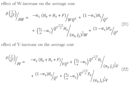
The effect of W-increase on the average cost

߲ ቀ

ொ^೅

ቁ

൘ ߲ܹ ൌ െן

ሺܪ

൅ ܪ

൅ ܨሻ

ܹܳ

൘ +ሺͳ െן

ሻܪ

ܳ

൘ + ቀ

െן

ቁ ܳ

భషן ן

ܪ

ሺן

ܬ

ሻ

ܹ

൙ + ሺͳ െן

ሻܲ

ܳ

൘ (21)

The effect of V-increase on the average cost

߲ ቀ

ொ^೅

ቁ

൘ ൌ ߲ܸ െן

ሺܪ

൅ ܪ

൅ ܨሻ

ܸܳ

൘ ൅ቀ

ן

െן

ቁ ܳ

భషן ן

ܪ

ሺן

ܬ

ሻ

ܸ

൙ + ሺͳ െן

ሻܪ

ܳ

൘ + ቀ

ן

െן

ቁ ܳ

భషן ן

ܲ

ሺן

ܬ

ሻ

ܸ

൙ (22)

6. Some results using cross-section data, and Discussion

The parameters of the production function with Douglas form and the main coefficients of equations (9)〜(22)are as follows (see Table 1 and Table 2).

5

An inquiry on the substitution of transportation-means (written in Japanese).

Table 1 The measured results of parameters in the production functions

parameters ln α

α

α

Ř

railroads 4.7047 (7.555)

1.0278 (20.391)

0.5077

(2.536) 0.9114 trucks 2.1824

(6.973)

0.9476 (23.723)

1.3045

(12.070) 0.9221 (Notes)The numerical value in parentheses shows t-value. Ř

represents an adjusted coefficient of

determination. We obtained the above results calculated on the freight traffic survey of Japan (published by Ministry of Land, Infrastructure, Transport and Tourism)in our previous research.

Skepticism to the Homotheticity, and Economies of Scale（Araki） −６ ７−

（ １ ５ ）

We can understand by equation (18)and (20)that the economies of scale work in the domestic freight industry because α (the total of space elasticity and velocity elasticity for output)is larger than unity. If α

is larger than α

, the production of output by the means of transport has a stronger advantage in the space-efficient factor (W)than in the velocity-efficient factor (V), and vice- versa. The transport by railroad is the former case and the one by truck is the latter case. Viewed from a different angle, the requirements of capital and of labor are more strongly affected by the space-efficient factor (W)rather than the time-efficient factor (V), and they have relatively high fixed-cost ratio. On top of that, the optimum capital-labor ratio varies along with the change of W and of V even under constant relative prices, because of the differences of W- elasticities and of V-elasticities for each input. The case of energy input relies more on the time-efficient factor (V)than on the space-efficient factor (W), and its cost is variable. Therefore we can ratiocinate by equations (18), (21) and (22)that scale-merits in combination with the fixed costs (H

, H

, F)have greater effect on the transport by railroad rather than on the one by truck. And the effects of V-increase on average-cost-reduction concerning labor and capital are greater than ones of W-increase. The reverse is the case of energy input.

On the other hand, we can also reason by the fourth-term each of right-hand side in equation (21), (22) that the opportunity-cost per weight (or per space)

Table 2 The key coefficients of main equations by means of transport

equation (16)(18)(20)(21)(21)(22)(22)

coefficient α (1−α) ／ α (1−α) ／ α

1−α

α

／ α −α

1−α

α

／ α −α

railroads 1.5355 −0.3487 −0.2271 −0.0278 −0.3584 0.4923 −0.1771 trucks 2.2521 −0.5560 −0.2629 0.0524 −0.5268 −0.3045 −0.7253 (Note)These coefficients are calculated by using results of parameters in Table 1.

−６ ８−

（ １ ６ ）

can be surely reduced not by W (the batch of load)-increase but by V (the velocity of each vehicle)-increase. In general, the productive activities with the development of high value-added-rate industries tend to depend all the more upon the time-efficient factor rather than the space-efficient factor. If we can consider price or value added per weight (or per space)as proxy variable of opportunity-cost per weight (or per space), the product of higher price (or of higher value added)per weight (or per space)should make the division of productive processes possible consequently in more extensive areas, with the velocity-increase of transport (or of transference).

7. Conclusion and Prospects

Many empirical studies have shown the existences of the economies of scale.

Those are mainly due to the dimensional differences arising from technological relationship between outputs and inputs basically. The scale (productive capacity)is the function of two types of elementary factors (i. e. the space- efficient factor and the time-efficient factor). The output-elasticities for all inputs are different from each other even under constant relative prices because of the differences in degree of choice between the two factors above and in the product-quality, which can have effects on each input-quantity. Therefore the existences of homotheticity between productive capacity and production factor

6

The reason is that the requirements of labor and capital inputs are a more strongly increasing function of W. On the other hand, the requirement of energy input is a more strongly increasing function of the running-distance (an increasing function of V). (See the second and third terms each of right-hand side in equation (21), (22).) Besides W-increase, it is necessary to shift to more energy-efficient productive methods to lower the input-coefficient of energy.

Skepticism to the Homotheticity, and Economies of Scale（Araki） −６ ９−

（ １ ７ ）

inputs (labor, capital, land etc.)are highly-improbable in the real economy.

Delving more deeply into the inquiry above, the degree of choice between the two basic factors above depends heavily upon the difference of opportunity-cost per space or per weight (a kind of quality of the product)for transportation (or for transference)in the same way as economic variables.

Acknowledgments

I would like to express my sincere appreciation and gratitude to the late Emeritus Professor Iwao Ozaki and the late Emeritus Professor Keiichiro Obi of Keio-Gijyuku University for their giving motives and hints to my research. And I also wish to thank Professor Mitsuo Takase of Fukuoka University for his valuable advice.

References

Beveren I. Van (2012)“Total Factor Productivity Estimation: A Practical Review,”

Journal of Economic Surveys, Vol.26.

Chad, Syverson (2011)“What Determines Productivity ?,” Journal of Economic Literature, Vol.49.

Chenery, Hollis B. (1953)“Process and Production Function from Engineering Data”, in Wassily W. Leontief, ed., Studies in the Structure of the American Economy, New York: Oxford University Press, Chap.8.

Christensen, Laurits R., Dale W. Jorgenson, and Lawrence J. Lau (1973)

“Transcendental Logarithmic Production Frontiers,” Reviewof Economics and Statistics, Vol.55.

Diewert, W.Erwin and T.J.Wales (1987)“Flexible Functional Forms and Global

7

Historically, the iron and steel production in the Great Leap Forward (1958- 61)by Mao Zedong is a well-known example which issue a denial of the homotheticity, the divisibility and the additivity of technology. Their traditional production-method enforced through gathering small-scale blast- furnaces resulted in failure respecting the quality of products. The homotheticity, the divisibility and the additivity of thechnology would be “The Emperor’s New Clothes”.

−７ ０−

（ １ ８ ）

Curvature Conditions,” Econometrica, Vol.55.

Haavelmo, Trygve (1944), “The Probability Approach in Econometrics”, Econometrica, vol.12, Supplement.

Hallak, J. Carlos. and Peter.K.Schott (2011)“Estimating Cross-Country Differences in Product Quality,” Quarterly Journal of Economics, Vol.126.

Julia, Roxana and Faye Duchin (2007)“World Trade as the Adjustment Mechanism of Agriculture to Climate Change,” Climate Change, Vol.82.

Kugler, Maurice and Eric Verhoogen (2012)“Prices, Plant Size, and Product Quality,” Reviewof Economic Studies, Vol.79.

Leontief, Wassily W. (1953)“Structural Change,” in Wassily W. Leontief, ed., Studies in the Structure of the American Economy, New York: Oxford University Press, Chap.2.

Leontief, Wassily W. (1970)“Dynamic Inverse,” in Anne P. Carter and Andrew Brody, eds., Contribution to Input-Output Analysis, Amsterdam: North-Holland.

Ozaki, Iwao. (1970), “Economies of Scale and Input-Output Coefficients,” in Anne P.

Carter and Andrew Brody, eds., Application of Input-Output Analysis, vol. Ⅱ, Amsterdam: North-Holland.

Skepticism to the Homotheticity, and Economies of Scale（Araki） −７ １−

（ １ ９ ）