Generalized C p Model Averaging for Heteroskedastic Models
Qingfeng Liu
∗Department of Economics, Otaru University of Commerce Revised Version
April 20, 2011
Abstract
This paper proposes a model averaging method, the generalized Mallows’ C
p(GC) method, which works well for heteroskedastic mod- els. Under some regularity conditions, we provide a feasible form of the GC method and show that the GC method has asymptotic optimality not only as a model averaging method but also as a model selection method for heteroskedastic models. We perform some Monte Carlo studies to investigate the small sample properties of the GC method.
The simulation results show that our method works well and performs better than alternative methods.
JEL classification: C51 C52
Keywords: Model Averaging, Model Selection, Asymptotic Opti- mality, Mallows’ C
p, Heteroskedastic error.
∗
Qingfeng Liu, Associate Professor, Department of Economics, Otaru University of
Commerce, 5-21, Midori 3-chome, Otaru, Hokkaido 047-8501, Japan. (Tel & Fax: +86
134 27 5312, E-mail: [email protected]).
1 Introduction
Model selection helps us to choose a single optimal model from a set of candi- date models. In the last two decades, model averaging has been proposed as an alternative to model selection. A model averaging estimator is obtained by taking the weighted average of the estimators obtained from candidate models. As compared to model selection, model averaging seeks to avoid selecting a very poor model and to improve the estimate with regard to risk. Model averaging methods can be separated into two groups: Bayesian model averaging methods and frequentist (non-Bayesian) model averaging methods. Bayesian model averaging methods have been advocated by many researchers (see Draper (1995), Hoeting, Madigan, Raftery, and Volinsky (1999), and Clyde and George (2004)). On the other hand, frequentist model averaging methods have a shorter history than their Bayesian coun- terparts. In the literature on frequentist model averaging methods, Buck- land, Burnham, Burnham, and Augustin (1997) proposed a smoothed-AIC (SAIC) based method and a smoothed-BIC (SBIC) based method, and Hjort and Claeskens (2003) proposed a frequentist model averaging method and derived the inference for the estimate based on the likelihood function of the model. Recently, Hansen (Hansen (2007), Hansen (2009), and Hansen (2010)) proposed several model averaging methods, which work for linear models, models based on series expansion, models with structural break, and models with a near unit root.
This paper extends Hansen (2007), which proposed a Mallows model
averaging (MMA) estimator for models with homoskedastic errors. The
weights of the models for the MMA estimator are determined by minimiz- ing a criterion similar to Mallows’ C
p(MC). Our extension is a generalization of the MMA method. The GC method works for both homoskedastic and heteroskedastic errors not only as a model averaging method but also as a model selection method. For heteroskedastic situations, Andrews (1991) showed asymptotic optimality for a model selection criterion based on MC.
However, Andrews (1991) did not provide a feasible form of this criterion, because of the difficulty associated with the consistent estimation of the co- variance matrix. We provide a way to avoid the estimate of the covariance matrix, and are thus able to propose a feasible form of the GC method.
Under some regularity conditions, we show that the GC method has asymp- totic optimality not only as a model averaging method but also as a model selection method for models with heteroskedastic errors.
The rest of this paper is organized as follows. In section 2, the GC method and its feasible form for model averaging and model selection are proposed, and the optimality of the GC method is discussed. In section 3, some simulation studies are performed to check the finite sample proper- ties of the GC method. Section 4 contains some concluding remarks. The appendix contains some technical proofs.
2 GC Method
Hansen (2007) proposed an MMA estimator. In his setup, the regressors are
assumed to be ordered, and the candidate regression models are assumed
to be nested. Wan, Zhang, and Zou (2010) extended the results of Hansen
(2007), by removing these assumptions. Our setup is similar to Wan, Zhang, and Zou (2010). The following is our model:
y
i= µ
i+ e
i, (1)
µ
i=
∑
∞ j=1θ
jx
ij,
E (e
i| x
i) = 0,
for i = 1, · · · , n, where y
iis a real-valued scalar, x
i= (x
i1, x
i2, · · · ) is a countably infinite real-valued vector, µ
iis assumed to be converging in mean square, and Eµ
2i< ∞ . Our results almost all are condational on x
i, for simplicity, we omit the conditinal expression in some cases hereafter.
The most important difference between our setup and that of Hansen (2007) and Wan, Zhang, and Zou (2010) is that in their setup, the error term e
iis assumed to be homoskedastic and not heteroskedastic as in our setup.
We assume that e
iis independent over i and E ( e
2i| x
i)
= σ
2i. The matrix form of the regressors is X ≡ (x
′1, x
′2, · · · )
′. The matrix form of eq.(1) is y = µ + e, where y = (y
1, · · · , y
n)
′, µ = (µ
1, · · · , µ
n)
′, and e = (e
1, · · · , e
n)
′. We propose the GC method to estimate µ
iwith a small risk (mean squared error, MSE).
The set of candidate models contains M models. The mth model has
k
m> 0 regressors that can be any variables in x
i. Note that we do not
restrict k
1< k
2< · · · < k
M, as is the case with the nested models assumed
in Hansen (2007). The mth approximating model of model (1) is
y
i=
km
∑
j=1
θ
j(m)x
ij(m)+ b
i(m)+ e
i, (2)
for m = 1, 2, · · · M , where x
ij(m)for j = 1, · · · , k
mdenotes the regressors in the mth model, and θ
j(m)denotes the coefficients. We thus have a matrix form of eq.(2):
Y = X
(m)Θ
(m)+ b
(m)+ e, (3) where Y = (y
1, · · · , y
n)
′, X
(m)is an n × k
mmatrix of the regressors with ij element x
ij(m)and with full column rank, Θ
(m)= (
θ
1(m), · · · , θ
km(m))
′, b
(m)= (
b
1(m), · · · , b
n(m))
′, and e = (e
1, · · · , e
n)
′. The LS estimator of Θ
(m)as derived from the mth model is ˆ Θ
(m)=
(
X
(m)′X
(m))
−1X
(m)′Y . The esti- mator of µ is
ˆ
µ
(m)= X
(m)(
X
(m)′X
(m))
−1X
(m)′Y ≡ P
(m)Y (4)
and the residual is ˆ e
(m)= Y − µ ˆ
(m). The model averaging estimator of µ is defined as
ˆ
µ (W ) =
∑
M m=1ω
(m)P
(m)Y ≡ P (W ) Y, (5) where W = (
ω
(1), · · · , ω
(M))
′is a weight vector in
H
n= {
W ∈ [0, 1]
M:
∑
M m=1ω
(m)= 1 }
. (6)
The setup of the weight vector is different from that in Hansen (2007) who
restricts the elements of the weight vector to be a/n, where a is some non- negative integers less than n, for the optimality of MMA.
Hansen’s MMA was designed for models with homoskedastic errors. Al- though it is hoped that it can also be applied to models with heteroskedastic errors, there does not exist any theoretical support for optimality and good performance in the heteroskedastic case. In this section, we propose the GC method for the heteroskedastic error case. We will show the optimality of this method and check its small sample performance in the next section.
The model averaging criterion is defined as follows:
GC
n= ∥ Y − P (W ) Y ∥
2+ 2tr [ΩP (W )] , (7)
where Ω is an n × n diagonal matrix with Ω
ii= σ
2i. Then, the estimator of the optimal weight vector is denoted as
W ˆ
GC= arg min
W∈Hn
GC
n. (8)
Our aim is to show the optimality of ˆ W
GCunder some regularity condi- tions. We define the loss function and the risk function as
L
n(W ) = ∥ µ ˆ (W ) − µ ∥
2(9)
and
R
n(W ) = E (L
n(W ) | X) , (10)
respectively. Then, optimality implies L
n( W ˆ
GCn)
inf
W∈HnL
n(W ) →
p1. (11) It can be easily seen that the expectation of GC
nis the sum of the risk func- tion and a constant. Hence, GC
ncan be regarded as an unbiased estimator of the risk function plus a constant.
Lemma 1 E (GC
n(W )) = R
n(W ) + ∑
ni=1
σ
i2.
The following theorem on the optimality of ˆ W
GCis an application of theorem 2.1* of Andrews (1991) and theorem 1’ of Wan, Zhang, and Zou (2010).
Theorem 2 For ξ
n≡ inf
W∈HnR
n(W ) and some integer 1 ≤ G < ∞ , if
E (
e
4Gi| x
i)
≤ κ < ∞ , (12)
M ξ
n−2G∑
M m=1( R
n(
W
m0))
G→ 0, (13)
and 0 < inf
iσ
i2≤ sup
iσ
2i< ∞ , then
Ln(
WˆGCn)
infW∈HnLn(W)
→
p1, where W
m0is a vector whose mth element is one and all other elements are zeros.
Andrews (1991) showed the asymptotic optimality for a model selection
method based on MC, but he did not propose a feasible criterion. The
difficulty in providing a feasible criterion arises from the fact that without
additional restrictions, one cannot expect to obtain a consistent estimator
of the covariance matrix Ω; since for heteroskedastic errors, Ω has at least
n parameters and we have only n observations. To solve this problem, our idea is to estimate not Ω but the scalar tr [ΩP (W )]. Using this approach, we propose the following feasible criterion for model averaging:
GC d
n≡ ∥ Y − P (W ) Y ∥
2+ 2
∑
n i=1ˆ
e
2ip
ii(W ) , (14)
where ˆ e
iis the residual from the largest model with the most number of regressors, and p
ii(W ) is the ith diagonal element of P (W ). Let ¯ e ≡ (˜ e
1, · · · , ˜ e
M) with ˜ e
mto be the n × 1 residual vector from the mth model, let ˆ Ω ≡ diag (
ˆ
e
2i, · · · , e ˆ
2n)
, and let Ξ ≡ (tr( ˆ ΩP
(1)), · · · , tr( ˆ ΩP
(M)))
′. Then we have the following expression
GC d
n= W
′¯ e
′eW ¯ + 2Ξ
′W (15)
The corresponding estimator of the optimal weight vector is W ˆ
GCdn
≡ arg min
W∈Hn
GC d
n. (16)
The following theorem shows that under some regularity conditions, if one replaces the term tr [ΩP (W )] in GC
nwith ∑
ni=1
ˆ e
2ip
ii(W ) as in eq.(14), Theorem 2 still holds as the following theorem claims.
Theorem 3 When ∑
ni=1
e ˆ
2ip
ii(W ) is used instead of tr [ΩP (W )], Theorem 2 is valid if
0 < lim n
−1∑
n i=1σ
i2= σ
2< ∞ , (17)
µ
′µ/n = O (1) , (18)
1≤
max
m≤Mmax
1≤i≤n
p
m,ii= O (
n
−1/2)
, (19)
˜ pe
′e
ξ
n→
p0, (20)
lim λ
max(n) = ∞ , (21)
log (λ
max(n)) = O (
n
1/2)
, (22)
where p ˜ ≡ sup
W∈Hnmax
1≤i≤n(p
ii(W )), λ
max(n) is the maximum eigen- value of X ˜
′X ˜ with X ˜ denoting the matrix of the regressors of the largest model, and p
m,iiis the ith diagonal element of P
(m).
In Li (1987), Andrews (1991), and Hansen and Racine (2010), there are some restrictions similar to (19), such as max
1≤m≤Mmax
1≤i≤np
m,ii→ 0.
Using some properties of P
(m), which is an idempotent matrix, one can show that such restrictions are reasonable, they exclude only extremely un- balanced models. If such restrictions do not hold, the variances of some ˆ µ
is, i.e., some elements of the estimate ˆ µ based on an unbalanced single model, will be extremely large, and as such, ˆ µ
is will be much less accurate.
It can be easily seen that if we restrict the weight vector to be W ∈ { i
1, i
2, · · · , i
M} , where i
iis a vector whose ith element is one and other ele- ments are zeros, then the GC method works as a model selection procedure to select a single model. The above two theorems are valid for this model selection procedure; further, this model selection procedure has optimality.
The criterion for model selection can be expressed as follows:
GC d
n(m) ≡ ∥ Y − P
mY ∥
2+ 2
∑
n i=1ˆ
e
2ip
m,ii. (23)
The estimator of the indicator of the optimal model can be obtained as follows:
ˆ
m ≡ arg min
1≤m<M
GC
n(m) . (24)
3 Monte Carlo Studies
To investigate the finite sample performance of our method, we conduct two Monte Carlo simulations. The number of replications is 1000 for both simulations. For comparison, not only the results of the GC method but also the results of the GCV (Liu (2010)), MMA (Hansen (2007)), SAIC and SBIC (Buckland, Burnham, Burnham, and Augustin (1997)), and AIC (Akaike (1973)) methods are shown. The GCV method is a model averaging method proposed by Liu (2010) in an unpublished paper, and is defined as
GCV
n(W ) = ∥Y − µ ˆ (W )∥
2(n − trP (W ))
2. (25)
The optimal weight vector selected by the GCV method is defined as W ˆ
GCV= arg min
W∈Hn
GCV
n(W ) . (26)
We have the DGP as
y
i=
∑
∞ j=1θ
jx
ij+ e
i. (27)
We cut off the infinite order at j = 30. The parameters are determined as in Hansen (2007): θ
j= c √
2αj
−α−1/2. We set the values as c = 0.2, 0.4, 0.6, · · · , 2
and α = 0.5. The parameter c affects the population R
2of eq.(27): R
2in- creases with c. The sample size is n = 150, the number of models is M = 10, and the biggest model has 10 regressors. For simplicity, in the simulations, we employ a nested setting: the (k + 1)th model is nested in the kth model.
x
ijs are independent over j, j = 1, · · · , m, and set to be i.i.d. N (0, 1) over i. The first simulation is with homoskedastic errors; we set e
ito be i.i.d.
N ( 0, σ
2)
, where σ = 1. In the second simulation study, we set e
ito be independent and heteroskedastic N (
0, σ
i2)
, where σ
i= x
2i2. Since the argu- ments in the above sections are restricted in the situation conditional on X, we first generate X and then fix the data of X through all the replications.
We define the sample MSE as M SE = 1/1000 ∑
1000i=1
(ˆ µ − µ)
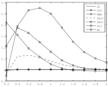
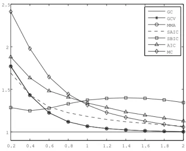
2, and calculate the MSE ratios (the ratios of the MSEs of the aforementioned methods and the MSE of the GC method). The MSE ratios are plotted in Figures I and II for homoskedastic and heteroskedastic errors, respectively.
We can see that the AIC method is dominated by the SAIC method for almost all values of c (R
2) in both simulations. The performance of the SBIC method is the worst in the homoskedastic case, but is better than some other methods for small values of c in the heteroskedastic case. The AIC method and the MC method perform moderately, and the GCV method and the MMA method are better than them in both cases.
The most important results are on the comparisons between the GC method and the GCV method and between the GC method and the MMA method. The GCV method is a perfect alternative to the MMA method;
both have almost the same MSE ratios. In the homoskedastic case, these
three methods have similar MSEs: the GC method performs slightly worse
than the GCV method and the MMA method when c < 0.4 but slightly bet- ter when c (R
2) is bigger. In the heteroskedastic case, the situation is much different. The GC method performs the best, and is particularly better than the GCV method and the MMA method when c is small. From these re- sults, we get that the GC method works well for models with heteroskedastic errors.
4 Conclusion
We proposed a model averaging method for heteroskedastic models. We ar- gued the optimality of this method, and performed Monte Carlo simulations to investigate its small sample properties. The results of these simulations show that the proposed method works well, particularly for models with heteroskedastic errors.
5 Appendix
Proof of Theorem 2. The proof of optimality in Wan, Zhang, and Zou (2010) is an application of Theorem 2 of Whittle (1960). Since Theorem 2 of Whittle (1960) holds even with heteroskedastic errors, when σ
2trP (W ) is replaced with trΩP (W ) and σ
2trP
2(W ) is replaced with trΩP
2(W ), the proof of Theorem 2 is almost the same as the proof of Theorem 1’ in Wan, Zhang, and Zou (2010).
Proof of Theorem 3. We denote the projection matrix of the largest
model as P
∗, and the ith diagonal element of P
∗as p
∗ii. We define ¯ P (W )
as a diagonal matrix which ith diagonal elemnt is p
ii(W ).
Condition (19) implies that ˜ p = O ( n
−1/2)
and the number of regres- sors in the largest model k
∗= O (
n
1/2)
; condition (13) implies that ξ
n→
∞. From the properties of an idempotence matrix, we have tr P ¯
2( W
m0)
≤ trP
2(
W
m0)
and 0 ≤ p
ii(W ) ≤ 1. We use C to denote some constant which could take different values in the following proof.
Since
GC d ≡ (Y − µ ˆ (W ))
′(Y − µ ˆ (W )) + 2
∑
n i=1ˆ
e
2ip
ii(W )
= GC + 2 (
n∑
i=1
ˆ
e
2ip
ii(W ) − tr [ΩP (W )]
)
, (28)
to prove Theorem 3, we only need to show that
sup
W∈Hn
{
∑
n i=1ˆ
e
2ip
ii(W ) − tr [ΩP (W )]
/
R
n(W ) }
→
p0. (29)
It can be easily seen that
sup
W∈Hn
{
∑
n i=1ˆ
e
2ip
ii(W ) − tr [ΩP (W )]
/
R
n(W ) }
≤ sup
W∈Hn
e ˆ
′P ¯ (W ) ˆ e − E (
e
′P ¯ (W ) e )/ ξ
n≤ sup
W∈Hn
{ e ˆ
′P ¯ (W ) ˆ e − e
′P ¯ (W ) e | + | e
′P ¯ (W ) e − E (
e
′P ¯ (W ) e )} /ξ
n≤ sup
W∈Hn
{ | e ˆ
′P ¯ (W ) ˆ e | + | e
′P ¯ (W ) e | + | e
′P ¯ (W ) e − E (
e
′P ¯ (W ) e )
| } /ξ
n≤ p ˜ { ˆ
e
′ˆ e + e
′e }
/ξ
n+ sup
W∈Hn
| e
′P ¯ (W ) e − E (
e
′P ¯ (W ) e )
| /ξ
n= ˜ p {
(µ + e)
′(I − P
∗) (µ + e) + e
′e } /ξ
n+ sup
W∈Hn
|e
′P ¯ (W ) e − E (
e
′P ¯ (W ) e )
|/ξ
n= ˜ p {
µ
′(I − P
∗) µ + 2µ
′(I − P
∗) e + e
′(I − P
∗) e + e
′e } /ξ
n+ sup
W∈Hn
| e
′P ¯ (W ) e − E (
e
′P ¯ (W ) e )
| /ξ
n≤ p ˜ {
µ
′(I − P
∗) µ + 2 | µ
′(I − P
∗) e | + e
′P
∗e + 2e
′e } /ξ
n+ sup
W∈Hn
| e
′P ¯ (W ) e − E (
e
′P ¯ (W ) e )
| /ξ
n. (30)
From conditions (13), (18), (19), and R
n(W ) ≥ µ
′(I − P (W )) µ, we have
˜
p µ
′(I − P
∗) µ
ξ
n≤
(
˜
p
2µ
′(I − P
∗) µ ξ
n2µ
′µ
)
1/2≤ (
˜
p
2R
n(W
0∗) ξ
n2µ
′µ
)
1/2= √
O (n
−1) o (1) O (n) → 0, (31)
where W
0∗is the weight vector giving weight 1 to the largest model.
Moreover, using similar techniques as in Wan, Zhang, and Zou (2010), i.e., by applying Chebyshev’s inequality, Theorem 2 of Whittle (1960) and R
n(W ) ≥ µ
′(I − P (W )) µ, denoting the ith element of µ
′(I − P
∗) as η
i, for any δ > 0, we have
P {
2˜ p | µ
′(I − P
∗) e | ξ
n> δ
}
≤ E (µ
′(I − P
∗) e)
24˜ p
2ξ
n2δ
2≤ C [
n∑
i=1
η
i2σ
i2]
1/2˜ p
2ξ
n2δ
2≤ C p ˜
2ξ
n2δ
2sup
1≤i≤n
σ
2iµ
′(I − P
∗) µ
≤ C p ˜
2ξ
n2δ
2R
n(W
0∗) → 0, (32) hence
2˜ p |µ
′(I − P
∗) e|
ξ
n→
p0. (33)
Moreover according to Lemma 1 of Lai and Wei (1982) and assumptions (21) and (22), we have
˜
p e
′P
∗e /ξ
n= O (
n
−1/2)
O (log λ
max(n)) o (1) a.s.
= O (
n
−1/2)
O (
n
1/2)
o (1) a.s. (34)
a.s.
→ 0. (35)
Furthermore, using Chebyshev’s inequality, Theorem 2 of Whittle (1960),
and C
m, m = 1, · · · , M , denoting some constant, for any δ > 0, we have,
P {
sup
W∈Hn
( e
′P ¯ (W ) e )
− E (
e
′P ¯ (W ) e ) /ξ
n> δ }
≤
∑
M m=1P {( e
′P ¯ ( W
m0)
e )
− E ( e
′P ¯ (
W
m0)
e ) > δξ
n}
≤
∑
M m=1E
{[( e
′P ¯ ( W
m0)
e )
− E ( e
′P ¯ (
W
m0) e )]
2Gδ
2Gξ
2Gn}
≤ δ
−2Gξ
n−2G∑
M m=1C
m{
n∑
i=1
p
2ii( W
m0) [
E (
e
4Gi)]
1/G}
G≤ max
1≤m≤M
(C
m) max
1≤i≤n
([ E (
e
4Gi)]
1/G)
δ
−2Gξ
n−2G∑
M m=1{
n∑
i=1
p
2ii(
W
m0) }
G= Cδ
−2Gξ
n−2G∑
M m=1[ tr P ¯
2(
W
m0)]
G≤ Cδ
−2Gξ
n−2G∑
M m=1[ trP
2(
W
m0)]
G= Cδ
−2Gξ
n−2G(
1≤
inf
i≤nσ
2i)
−G M∑
m=1
[ tr
{
1≤
inf
i≤nσ
i2IP
2(
W
m0)}]
G≤ Cδ
−2Gξ
n−2G(
1≤
inf
i≤nσ
2i)
−G M∑
m=1
[ tr { ΩP
2(
W
m0)}]
G≤ Cδ
−2Gξ
n−2G∑
M m=1[ R
n(
W
m0)]
G→ 0, (36)
where I is a n × n identity matrix. Therefore, we have sup
W∈Hn| (
e
′P ¯ (W ) e )
− E (
e
′P ¯ (W ) e )
|} /ξ
n→
p0. From the above results and eq.(20) we have
eq.(29). The proof of Theorem 3 is complete.
References
Akaike, H. (1973): “Information theory and an extension of the maxi- mum likelihood principle,” in Proc. of the 2nd Int. Symp. on Information Theory, ed. by P. B. N., and C. F., pp. 267–281.
Andrews, D. W. (1991): “Asymptotic optimality of generalized C
L, cross-validation, and generalized cross-validation in regression with het- eroskedastic errors,” Journal of Econometrics, 47, 359–377.
Buckland, S. T., C. Burnham, K. P. Burnham, and N. H. Augustin (1997): “Model selection: an integral part of inference,” Biometrics, 53, 603–618.
Clyde, M., and E. I. George (2004): “Model Uncertainty,” Statistical Science, 19(1), 81–94.
Draper, D. (1995): “Assessment and Propagation of Model Uncertainty,”
Journal of the Royal Statistical Society. Series B (Methodological), 57(1), 45–97.
Hansen, B. E. (2007): “Least Squares Model Averaging,” Econometrica, 75(4), 1175–1189.
(2009): “Averaging Estimators for Regressions with a Possible Structural Break,” Econometric Theory, 35(6), 1498–1514.
(2010): “Averaging Estimators for Autoregressions with a Near
Unit Root,” Journal of Econometrics, 158(1), 142–155.
Hansen, B. E., and J. Racine (2010): “Jackknife Model Averaging,”
Unpublished Working Paper.
Hjort, N., and G. Claeskens (2003): “Frequentist Model Average Esti- mators,” Journal of the American Statistical Association, 98, 879–899.
Hoeting, J. A., D. Madigan, A. E. Raftery, and C. T. Volinsky (1999): “Bayesian model averaging: a tutorial,” Statistical Science, 14(4), 382–417, with comments by M. Clyde, David Draper and E. I. George, and a rejoinder by the authors.
Lai, T. L., and C. Z. Wei (1982): “Least Squares Estimates in Stochas- tic Regression Models with Applications to Identification and Control of Dynamic Systems,” Annals of Statistics, 10(1), 154–166.
Li, K.-C. (1987): “Asymptotic Optimality for C
p, C
L, Cross-Validation and Generalized Cross-Validation: Discrete Index Set,” The Annals of Statistics, 15(3), 958–975.
Liu, Q. (2010): “Generalized CV and Generalized Cp Model Averaging,”
Unpublished Working Paper.
Wan, A. T., X. Zhang, and G. Zou (2010): “Least Squares Model Aver- aging by Mallows Criterion,” Journal of Econometrics, 156(2), 277–283.
Whittle, P. (1960): “Bounds for the Moments of Linear and Quadratic
Forms in Independent Variables,” Theory of probability and its applica-
tions, 5(3), 302–305.
0.2 0.4 0.6 0.8 1 1.2 1.4 1.6 1.8 2 0.9
1 1.1 1.2 1.3 1.4 1.5 1.6
GC GCV MMA SAIC SBIC AIC MC
Figure 1. MSE ratios of models with homoskedastic errors.
0.2 0.4 0.6 0.8 1 1.2 1.4 1.6 1.8 2 1
1.5 2 2.5
GC GCV MMA SAIC SBIC AIC MC