学位論文
Measurement of Charms and Bottoms with
Semi-leptonic Decay Modes in p+p Collisions at
s = 200 GeV
(重心エネルギー200GeVの陽子衝突における、
セミレプトニック崩壊モードを用いたチャームとボトムの測定)
平成25年12月博士(理学)
申請
東京大学大学院理学系研究科
物理学専攻
Measurement of Charms and Bottoms with
Semi-leptonic Decay Modes in
p+p Collisions at
√
s = 200 GeV
Ryohji Akimoto
Center for Nuclear Study,
Graduate School of Science,
University of Tokyo
A Dissertation Submitted in Partial Fullfillment of
the Requirements for the Degree of Doctor of Science
Abstract
A heavy quark is an interesting probe to understand a parton behavior in the ex-tremely hot and dense matter created by the relativistic heavy-ion collision. The heavy quarks are only produced in initial parton scattering in heavy-ion collisions due to their large masses. It means that the properties of the heavy quarks at the ini-tial stage of the heavy-ion collisions can be well described by those of p+p collisions. Therefore, the difference of the final states of the heavy quarks between the heavy-ion collisheavy-ions and p+p collisheavy-ions represents modificatheavy-ions during passing through the matter. The heavy quarks are expected to take longer time to equilibrate with the matter than light quarks since the energy loss of the heavy quarks is smaller than that of light quarks due to dead cone effect. Due to the long relaxation time, a history of interactions between the matter and the heavy quarks, which are strongly related to the properties of the matter, can be preserved in their diffusion during passing through the matter.
Since the energy loss depends on quark mass, the comparison of modifications during traveling in the matter between charm and bottom can test descriptions of the interaction. A new approach has been developed to evaluate the fraction of the bottom contribution in the heavy quark electrons. The fraction is evaluated by using the distances of the closest approach to the beam collision vertex, called DCA. DCA distributions of the electrons from charm and bottom decays have significantly different widths due to the difference of their life-times. The fraction can be evaluated by using the difference of their widths. Tracking with a good position resolution is necessary around a beam collision point to achieve the measurement. A silicon tracking system called VTX has been installed in PHENIX experiment in 2011 to achieve the precise tracking.
The bottom fraction has been evaluated at PHENIX experiment by the new ap-proach in p+p collisions with √s = 200 GeV at 1.5 < pT < 5 GeV/c. The bottom
fraction at pT < 2.5 GeV/c is succeeded to be measured for the first time. The
frac-tion at pT > 2.5 GeV/c is consistent with other results, and thus it is confirmed that
the evaluation by the new approach has been succeeded. The result can also provide a good test of perturbative QCD (pQCD) calculations. There is not a significant difference in differential cross sections of the electrons from charm and bottom decays between the predictions and measured results though center values of the predictions are ∼50% smaller than the measured results. The total cross section of the bottom production is also determined by extrapolating with FONLL calculations, and it is 3.41 ± 0.53 (stat) ± 2.14 (sys) µb. There is not a significant difference between the prediction and our result.
Contents
1 Introduction 1
1.1 Quark Gluon Plasma . . . 1
1.2 Heavy Quark . . . 2
1.3 Distance of Closest Approach . . . 4
1.4 Objective and Organization of Thesis . . . 6
2 Physics Background 7 2.1 Relativistic Heavy Ion Collision . . . 7
2.1.1 Space-Time Evolution . . . 7
2.1.2 Collision Geometry . . . 9
2.2 Heavy Quark . . . 12
2.2.1 Heavy Quark Production . . . 13
2.2.2 Fragmentation . . . 15
2.2.3 Semi-leptonic Decay . . . 17
2.3 Measurement of Heavy Quark . . . 18
2.3.1 Medium Modification . . . 18
2.3.2 Initial Modification . . . 19
2.3.3 Theoretical Description . . . 21
2.4 Separation of Charm and Bottom . . . 26
2.4.1 Correlation of Decay Products . . . 26
2.4.2 DCA Approach . . . 29
3 Experimental Setup 33 3.1 Relativistic Heavy Ion Collider (RHIC) . . . 33
3.2 PHENIX Detector Complex . . . 35
3.2.1 Detector Overview . . . 36
3.2.2 Magnet . . . 38
3.2.3 Beam-Beam Counter . . . 38
3.2.4 Drift Chamber . . . 42
3.2.5 Pad Chamber . . . 42
3.2.6 Ring Imaging Cherenkov Detector . . . 45
3.2.8 Silicon Vertex Tracker . . . 49
3.3 Data Acquisition . . . 56
3.3.1 Trigger . . . 56
3.3.2 Data Acquisition System . . . 57
4 Data Analysis 61 4.1 Overview of Data Analysis . . . 62
4.2 Track Reconstruction with Central Arm . . . 63
4.2.1 Track Reconstruction Technique . . . 64
4.2.2 Momentum Determination . . . 65
4.2.3 Analysis Variable . . . 67
4.3 Electron Identification . . . 67
4.3.1 Electron Identification with RICH . . . 68
4.3.2 Electron Identification with EMCal . . . 70
4.4 Track Reconstruction with VTX . . . 71
4.4.1 VTX Stand-alone Tracking . . . 72
4.4.2 CNT-VTX Tracking . . . 73
4.4.3 Track Fitting . . . 73
4.4.4 Beam Collision Vertex . . . 74
4.4.5 DCA Measurement . . . 77
4.4.6 Detector Alignment . . . 79
4.5 Event and Track Selection . . . 80
4.5.1 Event and Track Selection . . . 80
4.5.2 Isolation Cut . . . 81
4.6 Run Selection and Performance Stability . . . 83
4.6.1 Run Selection . . . 83
4.6.2 Performance Stability . . . 84
4.6.3 DCA Distribution of Inclusive Electron . . . 86
4.7 Simulation Tuning . . . 87
4.7.1 Detector Response . . . 87
4.7.2 Creation of Heavy Quark . . . 95
4.7.3 Trigger Efficiency . . . 100
4.8 Electron Yield . . . 101
4.8.1 Decay from Heavy Quark . . . 102
4.8.2 Decay from Light Mesons . . . 103
4.8.3 Photon Conversion . . . 104
4.8.4 Heavy Quarkonium . . . 108
4.8.5 Ke3 . . . 109
4.8.6 Hadron Contamination . . . 110
4.9.1 DCA Distribution . . . 121
4.9.2 Decay of Short-life Hadrons . . . 122
4.9.3 Decay of Long-life Hadrons . . . 124
4.9.4 Photon Conversion . . . 124
4.9.5 Hadron Contamination . . . 128
4.9.6 Fake Track Contribution . . . 129
4.10 Systematic Error Estimation . . . 132
5 Result 137 5.1 Fraction of Bottom Contribution . . . 137
5.2 Cross Section of Electrons from Charm and Bottom . . . 138
5.3 Total Cross Section of Bottom Production . . . 146
6 Discussion 149 6.1 Bottom Contribution in Heavy Quark Electron . . . 149
6.2 Comparison with Theoretical Prediction . . . 151
6.3 Cross Section of Bottom Production . . . 151
6.4 Future Perspectives of Heavy Quark Measurement . . . 151
6.4.1 DCA resolution . . . 155
6.4.2 S/N ratio . . . 156
7 Conclusion 159
List of Figures
1.1 The entropy density (s = !+p) over T3 as a function of T /T
ccalculated
by the lattice QCD. . . 3 1.2 An illustration of a D meson decay. . . 5 1.3 The interpolation for DCA calculation by using VTX hits. . . 5 2.1 A space-time picture of evolution of the matter created in a heavy ion
collision at RHIC. . . 8 2.2 A cartoon of central and peripheral collisions of nuclei with radii R. . 10 2.3 An illustration of the colliding nuclei before and after a collision in the
participant-spectator picture. . . 10 2.4 Npart and Ncollas a function of the impact parameter in Au+Au
colli-sion with √sN N = 200 GeV calculated based on the Glauber model. 11
2.5 Total multiplicity of charged particles at normalized by #Npart/2$ as a
function of Npart for √sN N = 19.6, 130, and 200 GeV, measured by
PHOBOS experiment. . . 12 2.6 The leading order and important the next leading order Feynman
di-agrams. . . 14 2.7 The pT distributions of B hadron measured in CDF with FONLL
pre-dictions in p+¯p collisions at√s = 1.96 TeV. . . 16 2.8 The differential cross sections of non-photonic electrons from heavy
quark measured in RHIC with FONLL predictions in p+p collisions at √s = 200 GeV. . . . 16 2.9 RAA and azimuthal anisotropy of the heavy quark electrons. . . 20
2.10 RAA of the heavy quark electrons for different pT ranges as a function
of the number of participantnucleons, and that of π0. . . . 21
2.11 Nuclear modification factor of the heavy quark electrons for d+Au and Au+Au collisions. . . 22 2.12 Modifications of charm and bottom cross-sections by the nuclear effects
of the PDFs calculated using the EKS 98 nuclear weight functions. . 22 2.13 A ratio of gluon emission spectra of charm and light quarks for quark
momenta pq = 10 GeV and 100 GeV. . . 23
2.14 η/s values as a function of temperature of medium evaluated by several interaction models. . . 26
2.15 RAAof electrons from heavy-quark decays in Au+Au with√s = 200 GeV,
and theoretical estimations by several models. . . 27
2.16 RAAs of electrons from charm and those from bottom for several inter-action models. . . 28
2.17 The fraction of the bottom contribution in the heavy quark electrons as a function of pT. . . 29
2.18 RMS values of DCA distributions of electrons from charm and bottom decays as a function of electron pT. . . 30
2.19 Examples of D meson and B meson decays. . . 31
3.1 The accelerator complex including RHIC at BNL. . . 34
3.2 Definition of the global coordinate system used in the PHENIX exper-iment. . . 37
3.3 Layout of the PHENIX detector configuration in the Run12. . . 39
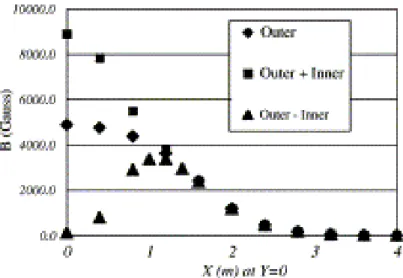
3.4 The field lines of the central magnet and muon magnets shown on a vertical cutaway drawing of the PHENIX magnets. . . 40
3.5 The field strength created by the CM with ++ and +− field configu-ration as a function of the distance from the beam axis. . . 40
3.6 Pictures of the BBC. . . 41
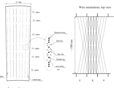
3.7 A frame of the drift chamber. . . 43
3.8 The layout of wire positions in a sector. . . 43
3.9 A schematic view of the PCs (PC1, PC2, PC3). . . 44
3.10 The pad and pixel geometry of the PC. . . 45
3.11 A cutaway view of RICH. . . 46
3.12 A schematic view of RICH cut along the beam axis. . . 47
3.13 Interior view of a lead scintillator calorimeter module showing a stack of scintillator and lead plates, wavelength shifting fiber readout and leaky fiber inserted in the central hole. . . 48
3.14 Exploded view of a lead glass calorimeter supermodule. . . 49
3.15 An Overview of a VTX arm. . . 51
3.16 A cross-sectional view of VTX and beam pipe. . . 52
3.17 A picture of a VTXP module. . . 52
3.18 A picture of a VTXS module. . . 53
3.19 A schmatic of the circuitry of ALICE1LHCB chip. . . 54
3.20 A schmatic view of a spiral-shape readout. . . 55
3.21 ADC distribution of X and U strips of VTX-stripixel detector. . . 55
3.22 The principal scheme of the electron trigger. . . 57
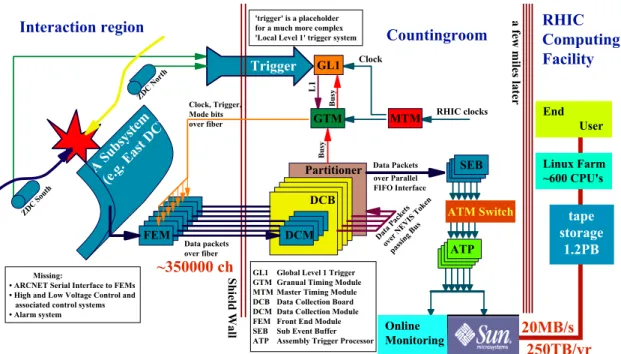
3.23 The schematic flow diagram of the data acquisition system. . . 59
4.1 Schematic views of a trajectory of a charged particle from the collision vertex to the DC in the x-y and r-z planes. . . 63
4.3 pT resolution of electrons as a function of pT evaluated by an
single-track simulation. . . 66
4.4 A schematic view of the definition of variables used for determination of the RICH variables . . . 68
4.5 rcor distribution and Np.e. distribution. . . 69
4.6 An illustration of a tracking with the VTX in x-y plane. . . 75
4.7 An illustration of a tracking with the VTX in r-z plane. . . 75
4.8 A distribution of the collision vertices of high multiplicity collisions of a run. . . 77
4.9 The beam center position as a function of run number. . . 78
4.10 The DCA resolution of electrons as a function of pT evaluated by a single-track simulation. . . 79
4.11 Residuals between an associated hit position and projection position at B0 in azimuthal and z directions. . . 80
4.12 The efficiencies for the e-ID cut and hadron selection of electrons and charged pions evaluated by a single-track simulations. . . 82
4.13 cdphi distributions of the electrons from π0 decays and charm elec-trons in a single-track simulation, and the distribution of the inclusive electrons in the data. . . 83
4.14 Widths of the distribution of the reconstructed collision vertices in x and y directions. . . 84
4.15 An illustration of a reconstructed path and an actual path. . . 85
4.16 Means and widths of DCA distributions of charged tracks for good runs. 86 4.17 Distribution of widths of DCA distributions of runs. . . 87
4.18 Ratios of entries at a tail and peak of a DCA distribution of each run and a distribution of the ratios normalized by their statistical errors. 88 4.19 A survival fraction after the isolation cut of each run and a distribution of the fractions normalized by their statistical errors. . . 88
4.20 DCA distributions of inclusive electrons and hadrons for pT > 1.5 GeV/c. 89 4.21 DCA distributions of electrons and positrons for pT > 1.5 GeV/c and a ratio of the DCA distributions as a function of DCA. . . 89
4.22 pT distributions of the electrons and charged pions in a single-track simulation and the MB data. . . 90
4.23 Distributions of the analysis variables related to the e-ID cut in the data and the simulation. . . 91
4.24 Distributions of chi-square components for CNT-VTX tracks with 3 associated hits in the data and simulation. . . 93
4.25 Distributions of chi-square components for CNT-VTX tracks with 4 associated hits in the data and simulation. . . 94
4.26 The DCA distributions of the inclusive electrons in all and the unstable runs, and their ratio as a function of DCA. . . 95
4.27 Distributions of dcphi of electrons in the data of the stable runs of a run group and in the simulation. . . 96 4.28 Distributions zed of electrons in the data of the stable runs of a run
group and in the simulation. . . 96 4.29 Distributions of components of chi-square for CNT-VTX tracks with 3
associated hits in the data and the simulation. . . 97 4.30 Distributions of components of chi-square for CNT-VTX tracks with 4
associated hits in the data and the simulation. . . 98 4.31 The invariant cross sections of charm and bottom in a simulation. . . 100 4.32 The trigger efficiencies of PbSc and PbGl as a function of pT. . . 101
4.33 The invariant cross section of the heavy-quark electrons and deviations from a modified Hagedorn function. . . 102 4.34 The total error, statistical error, and systematic error of the yield of
the heavy-quark electrons. . . 104 4.35 The invariant cross section of π0 with a fitting curve of modified
Hage-dorn function and deviations from the function. . . 105 4.36 The ratio of conversion electrons and electrons from π0 Dalitz decay. . 106
4.37 The pair-mass and φV distributions of e+-e− pairs. . . 108
4.38 The invariant cross section of J/ψ with a fitting curve of modified Hagedorn function and deviations from the function. . . 109 4.39 The distributions of dep for 1.5 < pT < 2.0 GeV/c. . . 111
4.40 Survival fractions for all electron sources. . . 113 4.41 A relative reconstruction efficiency of electrons as a function of pT. . . 115
4.42 The invariant cross sections of electrons from each source. . . 116 4.43 Yield ratios before the isolation cut. . . 117 4.44 Yield ratios after the isolation cut. . . 117 4.45 Hit distributions located close to associated hits to electron tracks. . . 119 4.46 Yields of the inclusive electrons of the data and the simulation after
the isolation cut. . . 120 4.47 The width of DCA distribution of hadrons as a function of pT. . . 123
4.48 The mean of the DCA distribution of the inclusive electrons as a func-tion of pT. . . 123
4.49 The DCA distributions of charm electrons with 1 < pT < 2 GeV/c
evaluated by a Gaussian convolution and by the PISA simulation, and their difference. . . 124 4.50 The DCA distributions of bottom electrons with 1 < pT < 2 GeV/c
evaluated by a Gaussian convolution and by the PISA simulation, and their difference. . . 125 4.51 An illustration of a reconstruction of conversion electrons. . . 126
4.53 The mean and RMS of the DCA distribution of the conversion electrons as a function of pT. . . 129
4.54 The DCA distribution of hadrons with and without dep cut. . . 130 4.55 The fractions of fake tracks in all electrons in the PISA simulation
as a function of pT for the electrons from π0 and η decays and the
conversion electrons. . . 131 4.56 The fraction of fake tracks in the inclusive electrons as a function of pT.132
4.57 The DCA distribution of the rotated fake tracks with pT > 1 GeV/c. 133
5.1 The fraction of the bottom contribution in the heavy quark electrons as a function of electron pT with FONLL calculation. . . 138
5.2 Fitting results of the DCA distribution of electrons with 1.5 < pT < 2.0 GeV/c
and a ratio between data and fitting result. . . 139 5.3 Fitting results of the DCA distribution of electrons with 2.0 < pT < 2.5 GeV/c
and a ratio between data and fitting result. . . 140 5.4 Fitting results of the DCA distribution of electrons with 2.5 < pT < 3.0 GeV/c
and a ratio between data and fitting result. . . 141 5.5 Fitting results of the DCA distribution of electrons with 3.0 < pT < 4.0 GeV/c
and a ratio between data and fitting result. . . 142 5.6 Fitting results of the DCA distribution of electrons with 4.0 < pT < 5.0 GeV/c
and a ratio between data and fitting result. . . 143 5.7 The differential invariant cross sections of the charm and bottom
elec-trons with FONLL calculations. . . 145 5.8 The cross sections of the heavy quark electrons of the result and the
simulation to create heavy quarks. . . 147 6.1 The fraction of the bottom contribution in the heavy quark electrons as
a function of pT in p+p collisions with√s =200 GeV with a theoretical
prediction. . . 150 6.2 The ratios of measured results and the FONLL calculation of charm
and bottom electrons as a function of electron pT. . . 152
6.3 The ratio of measured result at CDF and FONLL calculations of D mesons as a function of pT of the mesons. . . 153
6.4 The ratio of measured result at CDF and FONLL calculations of bot-tom hadrons as a function of pT of the hadrons. . . 153
6.5 The cross section of bottom production measured with several collision energies with a pQCD prediction. . . 154 6.6 An expected DCA resolution of electrons as a function of pT in Au+Au
collisions with 0-70% centrality evaluated with expected resolution of beam collision vertex, 15 µm, and DCA resolution shown in Fig. 4.10. 156 6.7 Survival fractions of conversion electrons, electrons from π0 decays,
and average of them. . . 157 6.8 An expected S/N ratio in Au+Au collisions. . . 158
List of Tables
2.1 Branching ratios and q-values for main semi-leptonic decay channels
of charm and bottom hadrons. . . 18
2.2 Life-times of charm and bottom hadrons. . . 31
3.1 Summary of the major design parameters of p+p with √s=200 GeV collisions at Year-2012 Run [1]. . . 35
3.2 Summary of the PHENIX detector complex. . . 38
3.3 Performance of pad chambers in Year-2002 and a cosmic ray test. . . 44
3.4 Summary of the basic parameters of the EMCal . . . 47
3.5 Major design parameters for the pixel detector. The maximum of the occupancies are evaluated with the multiplicity of central Au+Au col-lision with √sN N = 200 GeV. . . 50
4.1 The bit definition of quality. . . 65
4.2 Summary of the global and track variables used in this thesis. . . 67
4.3 Summary of the variables for electron identification. . . 67
4.4 Summary of the variables related to CNT-VTX tracks. . . 72
4.5 Requirements of rejection by the isolation cut. . . 83
4.6 A set of PYTHIA parameters used in this analysis. . . 99
4.7 Ratios of charm and bottom hadrons in PYTHIA. . . 99
4.8 Estimated hadron contamination in inclusive electrons. . . 111
4.9 A consistency between this estimation and the data with !corr p R0p . . . 127
4.10 The results of the Gaussian fitting of the DCA distribution of the rotated fake tracks. . . 133
4.11 Summary of systematic errors. . . 135
5.1 The result of the bottom fraction as a function of pT. . . 144
5.2 χ2/NDF of the DCA fitting. . . 144
5.3 χ2/NDF of the DCA fitting. . . 146
5.4 Branching ratios of bottom hadrons decaying into electrons. . . 148
Chapter 1
Introduction
1.1
Quark Gluon Plasma
Color confinement is one of the most interesting phenomena in the strong interac-tion. It is the phenomenon that a particle with a color charge can only exist in a color-singlet state, and a single quark is bound together into a color-singlet state, a meson or baryon. It is believed based on that a stable single quark has never been observed. Asymptotic freedom is supposed to be deeply related to the cause of color confinement. Asymptotic freedom is a feature of a non-abelian gauge theory. Quantum ChromoDynamics (QCD) is the theory of the strong interaction, and it is described by a non-abelian SU (3) gauge theory. Unlike Quantum ElectroDynamics (QED), the gauge bosons can interact each other in QCD as a consequence of the non-abelian gauge theory. Due to the self-interaction of the gauge bosons, the run-ning coupling constant of QCD decreases as the energy scale increases. This nature is called asymptotic freedom. The running coupling constant (αs) can be expressed
as a function of the momentum transfer (Q2) as follows.
αs∼
12π
(33 − 2Nf) log (Q2/ΛQCD)
, (1.1)
where Nf is the number of quark flavors, ΛQCD ∼ 0.2 GeV is the QCD scale. The
asymptotic freedom suggests a possibility that color confinement can be broken in an extremely high temperature or high density, i.e. a phase transition occurs from the confined state (ordered phase) to the deconfined state (disordered phase). The deconfined state is called Quark Gluon Plasma (QGP) [2].
Lattice QCD calculations, which is a numerical approach based on the first princi-pal, predict that the phase transition occurs at a critical temperature, Tc & 170 MeV
or the transition energy density !c & 1 GeV/fm3[3, 4, 5]. Figure 1.1 shows the entropy
density (s = ! + p) over T3 as a function of T /T
c calculated by the lattice QCD [6].
The entropy density increases rapidly around at Tc ∼ 170 MeV due to the increase
High-energy heavy-ion collision is expected to be a powerful and unique tool to achieve very high temperature and density which are enough to create QGP [7, 8]. There have been many attempts to produce QGP experimentally from heavy-ion collisions. The experiments of heavy-ion collisions began at Bevalac at Lawrence Berkeley National Laboratory (LBNL) with ∼2A GeV and a fixed target in the middle of 1970’s, then followed in Alternating Gradient Synchrotron (AGS) at Brookhaven National Laboratory (BNL) and in Super Proton Synchrotron (SPS) at European Laboratory for Particle Physics (CERN). Currently, heavy-ion collision experiments have been performed with Relativistic Heavy Ion Collider (RHIC) at BNL and Large Hadron Collider (LHC) at CERN. RHIC and LHC can collide heavy nuclei with the center-of-mass energy per nucleon pair up to 200 GeV and 2.76 TeV, respectively.
There are a lot of indications that a new state of matter is formed [9, 10, 11, 12]. Major experimental findings at early stage of RHIC experiments are a suppression of jets at heavy-ion collisions by comparing with p+p collisions [9, 10], which indicates formation of high density matter, and a large azimuthal anisotropy in non-central heavy-ion collision, which can be successfully described by a relativistic hydrodynam-ics model [11, 12]. Studies of the properties of the matter by the experiments of heavy-ion collision have a difficulty due to the fact that the matter undergoes several stages during its space-time evolution, as is described in Sec. 2.1.1. Since observables are measured through measurements of particles after the space-time evolution, they are affected by integrated information of the interaction with the matter. Therefore, the studies of the properties are necessary to be carried out with multiple probes with different features.
1.2
Heavy Quark
Heavy quarks (charm and bottom) are only produced in initial parton scatterings due to their large masses, and their initial states can be understood well from the measurements of p+p collisions. In addition, the momentum transfer to create the heavy quarks is much larger than ΛQCDdue to their large masses, and thus, it leads to
αs ∼ 0.3, which is enough small to apply perturbative QCD (pQCD) to calculate the
production of the heavy quarks. Therefore, the measurements of charm and bottom productions in p+p collisions can provide a good test of pQCD calculations.
The energy loss of the heavy quark is smaller than that of light quarks due to dead cone effect [13], and thus, the heavy quark is not expected to fully equilibrate with the matter, which is different from light quarks. The thermal relaxation time of the heavy quarks has been argued to be larger than that of light quarks by a factor of mHQ/T [14], where mHQis a mass of heavy quarks and T is a typical temperature
of the matter. Due to the long relaxation time, the heavy quarks serve as impurities in the thermalizing matter, and a history of interactions between the matter and
Figure 1.1: The entropy density (s = ! + p) over T3 as a function of T /Tc calculated by
In order to extract the properties of the matter, understandings of the interac-tion between the heavy quarks and the matter are necessary. Since the energy loss depends on quark mass, the comparison of modifications during traveling in the mat-ter between charm and bottom is expected to provide detail information about the interaction.There are results about charm and bottom measurement in p+p colli-sions [15, 16]. However, the results are only for high-pT region and the approaches
employed to extract the results are hard to be employed for heavy-ion collisions due to a large background derived from a high multiplicity condition of heavy-ion colli-sions. The difficulty to employ the approaches in heavy-ion collisions is discussed in Sec. 2.3.
1.3
Distance of Closest Approach
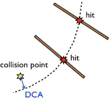
The distance of the closest approach (DCA) to a beam collision vertex is utilized to extract charm and bottom signals in this thesis. Figure 1.2 illustrates a decay of a D meson (D → e + K + ν). A D meson is created by a beam collision, and proceeds and decays far from the collision point. An electron is ejected by the decay. DCA of the electron track is the distance between the track, which is represented as the red arrow in Fig. 1.2, and collision point. Without a magnetic field, the DCA can be written by d · sin θ, where d is the distance between the decay point and the beam collision point, and θ is the angle difference between the tracks of D meson and electron. Therefore, DCA depends on the life-time of a mother particle and the q-value of a decay mode. Yields of charm and bottom can be evaluated by using the difference of their life-times. The analysis with the DCA is called “DCA approach”. Details of the approach are written in Sec. 2.3 and chapter 4.
The DCA is calculated by interpolating from a detector hit point taking account of a bending in a magnetic field. The interpolation is peroformed by assuming a track path is a circle. The PHENIX detector complex has spectrometers which can measure momenta with good precision. However, the resolution of the interpolation is not good since the spectrometers locate far from the beam path (220 cm). A silicon tracking system called VTX has been installed for the DCA measurement in the PHENIX detector complex for the DCA measurement. The VTX enable to measure tracks around beam collision points with a good precision. Two panels of Fig. 1.3 illustrate the interpolation by using VTX hits. The VTX is a barrel detector with 4 barrels surrounding the beam path. The innermost barrel locates at 2.6 cm far from the beam path and its position is 14 µm and 152 µm for directions perpendicular and parallel to the beam path, respectively [17]. Details of the VTX is written in Sec. 3.2.8.
Here, the definition of the DCA used in this thesis is given. The DCA is calculated in 2-dimensional plane perpendicular to the beam path, i.e. a track is projected in
Figure 1.2: An illustration of a D meson decay (D → e + K + ν).
ignored in the calculation of the DCA, and thus, the DCA calculated in 3-dimensional space is not exactly the same as the DCA used in this thesis. The sign of the DCA is defined by an alignement of the projected track and beam collision point. A track of a charged particle is rotated by a magnetic field. When the beam collision point is inside to rotation circle, its DCA is positive. Otherwise, it is negative. The left and right panels of Fig. 1.3 show tracks with positive and negative DCA, respectively.
1.4
Objective and Organization of Thesis
The fraction of electrons∗ from bottom decay in the electrons from charm or bottom
decays in p+p collisions with√s = 200 GeV is measured from the DCA approach in this thesis. By combining a published result of the cross section of the electrons from charm or bottom decays [18], the cross section of the electrons from charm decays and that of bottom decays are evaluated. The cross sections are important since they can provide information of initial condition of the heavy quarks in heavy-ion collisions and they are used as a reference for spectra of the heavy quark in heavy-ion collisions. In addition, the measurements of charm and bottom productions in p+p collisions can provide a good test of pQCD calculations.
The organization of this thesis is as follows. In chapter 2, theoretical and experi-mental backgrounds are described. In chapter 3, the RHIC accelerator complex and the PHENIX detectors are described. In chapter 4, the analysis of the DCA approach to extract the fraction of electrons from bottom decay in the electrons from charm or bottom decays is explained. In chapter 5, the fraction of the bottom contribution, the differential invariant cross section of the electrons from charm and bottom de-cays, and the total cross section of bottom production are shown. In chapter 6, the interpretations of the results are discussed. Chapter 7 is the conclusion of this thesis.
Chapter 2
Physics Background
In this chapter, theoretical and experimental backgrounds of our work are described. At first, the picture and description of high-energy heavy-ion collisions in Sec. 2.1. These are necessary to understand results of the heavy-ion collision experiments. In Sec. 2.2 and Sec. 2.3, theoretical descriptions and experimental results about heavy quarks are described. The electrons from heavy-quark decay have been measured in our work. Theoretical descriptions of the production, hadronization, and decay of heavy quarks are summarized in Sec. 2.2. Experimental results about heavy quarks in heavy-ion collisions and their theoretical interpritations are described in Sec. 2.3.
2.1
Relativistic Heavy Ion Collision
A relativistic heavy-ion collision is a unique tool to create an extremely hot and dense matter. Several collider experiments have been performed by using RHIC and LHC in order to study the QGP.
A heavy-ion collision experiment began at Bevalac at Lawrence Berkeley Na-tional Laboratory (LBNL) with ∼2A GeV and a fixed target in the middle of 1970’s. Then experiments were carried out in Alternating Gradient Synchrotron (AGS) at Brookhaven National Laboratory (BNL) and in Super Proton Synchrotron (SPS) at European Laboratory for Particle Physics (CERN). Their beam energies were 14A GeV and 160A GeV, respectively. Currently, heavy-ion collision experiments have been performed with Relativistic Heavy Ion Collider (RHIC) at BNL and Large Hadron Collider (LHC) at CERN. RHIC and LHC can collide heavy nuclei with the center-of-mass energy per nucleon pair up to 200 GeV and 2.76 TeV, respectively.
2.1.1
Space-Time Evolution
The matter created by relativistic heavy-ion collisions undergoes a space-time evolu-tion. The evolution of the matter is expected to be described based on the scenario proposed by J.D. Bjorken [19]. It is assumed that the space-time evolution depends on
only the proper time τ =√t2− z2 in the high energy limit in the scenario. Figure 2.1
shows a space-time picture of the evolution of the matter created in the heavy-ion collision with the longitudinal coordinate z and the time coordinate t. The space-time evolution can be separated into mainly the following four different phases separated by the dotted lines in Fig. 2.1:
Figure 2.1: A space-time picture of evolution of the matter created in a heavy ion collision
at RHIC. The proper times τ and temperatures T for different phases are expected from a hydrodynamical model [20]. The mixed phase would exist only if the transition is first order.
1. Pre-equilibrium (τ = 0 ∼ τ0)
Two incoming nuclei collide each other and many parton collisions take place. Incoming partons lose their kinematic energy by the collisions, and a large amount of energy is deposited at a tiny colliding region. A lot of secondary particles are produced in the region. The secondary particles subsequently interact with each other and the system is led to a local equilibrium.
2. Deconfined partonic phase (QGP) in thermal equilibrium (τ = τ0∼ τC)
3. Mixed phase between QGP and hadrons (τ = τC ∼ τH)
When the system cools down to the transition temperature TC, a phase
tran-sition is taken place from the QGP to a phase of ordinary hadronic matter. A hadronization starts, and the mixed phase consisting of the quarks, gluons, and hadrons is made.
4. Hadron gas (τ = τH ∼ τF)
The system finishes hadronization. The produced hadrons keep interacting with each other until the system cools down to the kinematic freeze-out temperature TF.
We never know where each of observed particles is generated. It leads our study to understand properties of QGP difficult since measured particles are affected by inte-grated information of the interaction with a matter at each of the stages. Therefore, it is important to study the properties with multiple probes with different features.
2.1.2
Collision Geometry
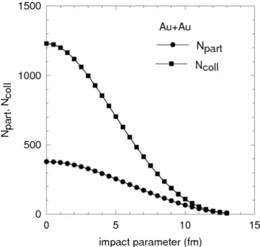
The collision geometry of the heavy-ion collisions play an important role in colli-sion dynamics, and thus, important to interpret observed results. The participant-spectator picture is a simple geometrical picture characterizing the collision with the impact parameter, b, which is shown in Fig. 2.2. Figure 2.2 illustrates central (left) and peripheral collisions (right) of nuclei with radii R. The central (peripheral) colli-sion is a collicolli-sion with small b (large b). As shown in Fig. 2.3, incoming nuclei look like a thin pancake due to the Lorentz contraction. When b > 2R, where R represents the radius of the nuclei, the incoming nuclei interact mainly by the electromagnetic force. As b decreases, the nuclei geometrically overlap, then an effect by the strong in-teraction suddenly increases. When b < 2R, the nucleons in the nuclei are classified into two groups: the participant, which is in the overlapping region, and the specta-tor, which is not. Since the spectator keeps its longitudinal velocity and emerges at nearly zero degrees in the collisions, it is relatively easy to separate the spectator and participant experimentally. The relations between the impact parameter, centrality, the number of participants (Npart), and the number of binary collisions (Ncoll) are
obtained based on Glauber model [21, 22]. Figure 2.4 shows Npartand Ncollas a
func-tion of the impact parameter in Au+Au collision with √sN N = 200 GeV calculated
based on the Glauber model [23].
Particle Production
Ncolland Npartare important parameters for particle production in heavy-ion collision.
Particle production in soft processes is expected to be proportional to Npart, and that
in hard processes is expected to be proportional to Ncoll. Figure 2.5 shows total
Figure 2.2: A cartoon of central (left) and peripheral (right) collisions of nuclei with radii R.
Figure 2.3: An illustration of the colliding nuclei before (left) and after (right) a collision
Figure 2.4: Npartand Ncollas a function of the impact parameter in Au+Au collision with
√s
N N = 200 GeV calculated based on the Glauber model [23]. Inelastic nucleon+nucleon
cross section (σN N) and nuclear charge density (ρ(r)) are assumed to be σN N = 42 mb
measured by PHOBOS experiment [24]. The normalized total multiplicity of charged particles, which is dominated by particles produced by soft processes, is constant, and thus the total multiplicity is scaled by Npart, from peripheral to central collisions. As
is described in Sec. 2.2, heavy quarks are produced by hard processes, and integrated yield of electrons from heavy quark decays is proportional to Ncoll. In order to quantify
effects from the matter created by heavy-ion collisions on particle produced by hard processes, following nuclear modification factor (RAA) is utilized:
RAA = dNAA/dpT Ncoll· dNpp/dpT . (2.1) part
N
0
200
400
〉
/2
partN〈
/
chN
0
10
20
30
-e + e p p pp/ PHOBOS p inelastic p pp/ 19.6 GeV 130 GeV 200 GeVFigure 2.5: Total multiplicity of charged particles at normalized by #Npart/2$ as a function
of Npart for √sN N = 19.6, 130, and 200 GeV, measured by PHOBOS experiment [24].
2.2
Heavy Quark
The heavy quarks are only produced in initial parton scattering in heavy-ion collisions due to their large masses. It means that the properties of the heavy quarks at the initial stage of the heavy-ion collisions can be described by those of p+p collisions, and thus, the difference of the final states of the heavy quarks between the
heavy-Measurement of heavy quarks are performed with decay electrons. Heavy quark production, hadronization (fragmentation), and decay are described in following sec-tions. Decay modes of heavy quarks with a lepton in decay products are called semi-leptonic decay modes. In this thesis, semi-semi-leptonic decay modes with an electron in decay products are simply called semi-leptonic decay modes.
2.2.1
Heavy Quark Production
The energy scale for the production of heavy quarks Q2
∼ M2
c(b) is much higher
than ΛQCD, and thus, the coupling constant αs is ∼ 0.3. It is small enough to apply
the perturbative QCD (pQCD) calculation for the production of heavy quarks. The general perturbative calculation for the total cross section of quark-antiquark pair production by a parton scattering can be expressed by the following equation.
σij(ˆs, MQ2, µ2R) = α2 s(µ2R) M2 Q inf ! k=0 (4παs(µ2R))k k ! l=0 fij(k,l)(η) " ln # µ2 R M2 Q $%l , (2.2) where µ2
R is called renormalization scale, which is a order of the square of the quark
mass, M2
Q, and ˆs is the center-of-mass energy of the parton scattering. The
dimen-sionless parameter η = ˆs/M2
Q − 1 reflects the phase space of the heavy quark pair
production (√s should be at least 2Mˆ Q to create aquark-antiquark pair). i and j
are the indices of parton, and they correspond to q, ¯q, or g. fi,j(k,l) is a dimensionless scaling function representing the amplitude of a partonic scattering diagram. k repre-sents the order of the process diagram. k=0 corresponds to the Leading-Order (LO) and k=1 corresponds to the Next-Leading-Order (NLO). Figure 2.6 shows Feynman diagrams of LO and important NLO process. The total cross section for heavy quark production can be calculated in p+p collisions with a parton distribution function (PDF) in protons, σij(ˆs, MQ2, µ2R), as follows: σpp(s, MQ2, µ 2 R, µ 2 F) = ! i,j=q,¯q,g & 1 4M2 Q/s dτ & τ dx1 x1 Fip(x1, µ2F)F p j(τ /xi, µ2F)σij(τ s, MQ2, µ 2 R). (2.3) µ2
F is a momentum transfer scale (factorization scale) of the PDF factorization.
Fip(x1, µ2F) is a PDF in term of a momentum fraction, x1, and factorization scale.
Eq. 2.3 have three free parameters, M2
Q, µ2R and µ2F. The uncertainty of the
pertur-bative calculation is usually determined by varying these parameters.
Fixed-Order plus Next-to-Leading-Log Calculation
Fixed-Order plus Next-to-Leading-Log (FONLL) calculation is the theory based on pQCD calculation about heavy quark production [25, 26]. FONLL can be compared
(a)
g
g
Q
Q
(b)
q
q
g
Q
Q
(c)
g
g
Q
Q
g
(d)
g
g
Q
Q
g
(e)
g
g
g
Q
Q
g
(f)
g
g
g
Q
Q
g
g
Figure 2.6: The leading order and important the next leading order Feynman diagrams.
(a) gluon fusion. (b) quark-antiquark annihilation. (c) pair creation with gluon emission. (d) flavor excitation. (e) gluon splitting. (f) gluon splitting with excitation character.
directly with the experimental results. The differential invariant cross section of the heavy-quark hadrons can be written as follows:
Ed
3σl
dp3 = E
HQd3σHQ
dp3 ⊗ D(Q → HHQ), (2.4)
where the symbol ⊗ denotes a generic convolution, the leptonic decay spectrum term f (HHQ→ l) also implicitly accounts for the proper branching ratio and D(Q → HHQ)
denotes fragmentation process. The distribution of heavy quarks, EHQd3σHQ/dp3 is
evaluated at the Fixed-Order plus Next-to-Leading-Log (FONLL) level pQCD cal-culation. FONLL includes the full fixed-order NLO result (FO) and re-summation perturbative terms proportional to αn
s(log k(p
T/m)) to all orders with next-to-leading
logarithmic (NLL) accuracy (i.e. k = n, n−1), where m is mass of heavy quark. The NLL terms take an important role to converge of the perturbative series for high pT (pT > m) region. Heavy quark fragmentation is implemented within the
FONLL formalism that merges the FO + NLL calculations. The NLL formalism is used to extract the non-perturbative fragmentation effects from the experimental data in e+e− collisions using Mellin transforms [27]. Figure 2.7 shows the p
T
distri-butions of B hadron measured in CDF with FONLL predictions in p+¯p collisions at √s = 1.96 TeV [28]. Figure 2.8 shows the differential cross sections of non-photonic electrons from heavy quark measured in RHIC with FONLL predictions in p+p col-lisions at √s = 200 GeV. The red and blue points represents the cross sections reported from PHENIX and STAR experiments [15, 29]. The solid line represents the central value of the FONLL calculation, and the dash line represents its uncer-tainty. FONLL calculation provides a successful description for the experimental pT
distributions of heavy quark. However, there is large theoretical uncertainty for the absolute value of cross section at FONLL. For example, FONLL predicts the total cross section of charm, σc¯c to be 256+400−146 µb and the total cross section of bottom, σb¯b
to be 1.92+1.21
−0.78 µb in p+p collisions a
√s = 200 GeV.
2.2.2
Fragmentation
Heavy quarks created by parton scatterings pick up light quarks in order to create color singlet hadrons, which is called as fragmentation process. The differential cross section of heavy quark hadrons (dσH/dpH
T) can be written as follows:
dσH dpH T = & d ˆpTdz dσHQ d ˆpT DHHQ(z)δ(pHT − z · ˆpT), (2.5)
where ˆpT is the transverse momentum of heavy quarks and pHT is the transverse
mo-mentum of heavy quark hadrons. dσHQ/d ˆp
T is the differential cross section of heavy
quarks, and z is the momentum fraction of the heavy quark carried by the hadron. DH
Figure 2.7: The pT distributions of B hadron measured in CDF with FONLL predictions in p+¯p collisions at√s = 1.96 TeV.
[GeV/c]
Tp
2
4
6
8
]
3c
-2[mb GeV
3/dp
σ
3E d
-910
-810
-710
-610
-510
-410
PHENIX
STAR
FONLL
Figure 2.8: The differential cross sections of non-photonic electrons from heavy quark
measured in RHIC with FONLL predictions in p+p collisions at √s = 200 GeV. The red
and blue points represents the cross sections reported from PHENIX and STAR experi-ments [15, 29]. The solid line represents the central value of the FONLL calculation, and
producing hadron with given momentum fraction (z). The fragmentation function of heavy quarks should be much larger than that of a light hadron. In the limit of a very heavy quark, one expects that the fragmentation function for a heavy quark to go into any heavy hadron to be peaked near 1. The fragmentation function can be split into a perturbative part and an non-perturbative part. Non-perturbative effect in the calculation of the heavy quark fragmentation function is performed in prac-tice by convolving the perturbative result with a phenomenological non-perturbative form. There are various parameterizations for the non-perturbative part which have free parameters. The free parameters in the non-perturbative parameterizations are determined by the experimental results in e+e− collisions based on the assumption
that the fragmentation function is independent on how to be produced. In general, the parameters in the non-perturbative forms do not have any absolute meaning, since these depend on the order of the perturbative calculation in the fragmentation function. The most accurate approach to derive the fragmentation function is to use the Mellin transforms of the fragmentation function and obtain the momenta of this transform from the experimental data. The treatment of the fragmentation process discussed above is expected to be valid in p+p collisions. In the case of heavy-ion collisions, the coalescence process becomes important in the fragmentation of heavy quark.
2.2.3
Semi-leptonic Decay
There are two merits in the measurement via decay electrons with PHENIX detector comparing to a full reconstruction of a hadronic decay with all decay products: one is a large branching ratio and the other is a good signal-to-noise (S/N) ratio. Total branching ratio of semi-leptonic modes are around 10% for both charm and bottom. Branching ratios of main semi-leptonic decay modes are summarized in Tab. 2.1. On the other hands, a specific mode of hadronic decay modes is small, especially for bottom. Branching ratios of hadronic decay modes of B meson is ∼10−4. A S/N
ratio of electrons from heavy-quark decays is achieved ∼1 at pT > 1.5 GeV/c, as is
described in Sec. 4.8.8. However, there is a disadvantage that measured electrons are sum of charm and bottom decays, and thus, an additional information is necessary to separate yields of charm and bottom decays. Contributions of charm and bottom decays are evaluated by using a DCA distribution in this thesis.
For processes where the momentum transfer is much less than the W boson mass, the amplitude of a semi-leptonic decay of a quark, Q, to another one, q (YQq! → Xqq!+
l + ν), can be given by M (YQq! → Xqq! + l + ν) = i GF √ 2VqQL µH µ, (2.6)
where GF is the Fermi constant of the weak interaction and VqQ is an element of the
Cabibbo-Kobayashi-Maskawa (CKM) matrix. Lµ is the leptonic current and H µ is
the hadronic current. Hµ is difficult to calculate from first principles since it includes
non-perturbative QCD effect. The hadronic current is usually parameterized with form factors.
Table 2.1: Branching ratios and q-values for main semi-leptonic decay channels of charm
and bottom hadrons.
hadron decay channel branching ratio q-value D+ → e+K0ν e 8.83±0.22% 1.37 GeV D+ D+ → e+K∗0ν e 3.68±0.21% 0.97 GeV D0 → e+K−ν e 3.55±0.05% 1.37 GeV D0 D0 → e+K∗−ν e 2.17±0.16% 0.97 GeV Ds→ e+φνe 2.49±0.14% 0.97 GeV Ds Ds → e+ηνe 2.67±0.29% 1.42 GeV Ds → e+η#νe 0.99±0.23% 1.01 GeV Λc Λc → e+Λνe 2.1±0.6% 1.17 GeV B+ → e+D0ν e 2.23±0.11% 3.41 GeV B+ B+ → e+D∗0ν e 5.68±0.19% 3.27 GeV B0 → e+D−ν e 2.17±0.12% 3.41 GeV B0 B0 → e+D∗−ν e 5.01±0.12% 3.27 GeV Bs Bs → e+DsνeX 7.9±2.3% -Λb→ e−Λcνe 5.0+1.9%-1.4% 3.33 GeV Λb Λ b → e−Λcπ+π−νe 5.6±3.1% 3.05 GeV
2.3
Measurement of Heavy Quark
Measurements of heavy quarks have been carried out at several species of beam col-lision systems (p+p, d+A, and A+A) and RHIC and LHC [18, 30, 29, 31]. In this section, these results are described. In addition, understandings of interaction be-tween heavy quarks and the matter created by heavy-ion collisions from the results are described.
2.3.1
Medium Modification
Medium modification of heavy quarks is studied by the measurement of the heavy quark electrons in A+A collisions. Figure 2.9 show RAA for 0-10% central (most
strong suppression at high pT and a large azimuthal anisotropy have been observed in
Au+Au collisions. It indicates that the heavy quarks as well as light quarks strongly interact with the matter created in A+A collisions. RAA at high pT is almost same
level as π0. However, the complete understanding of the parton behavior in the QGP,
which is essential to extract QGP properties, is still a challenging task since the mechanism of the energy loss is different between light and heavy quarks, as is shown in Sec. 2.3.3.
Figure 2.10 shows RAA of the heavy quark electrons for different pT ranges as a
function of the number of participant nucleons, Npart [18]. As is shown in Fig. 2.4,
larger Npart means smaller impact parameter, i.e. more central collision. The green
and blue circles are for the heavy quark electrons with pT > 0.3 GeV/c and with
pT > 3.0 GeV/c, respectively. The red points are for π0 with pT > 4.0 GeV/c. For
the integration interval pT > 0.3 GeV/c containing more than a half of the heavy
quark electrons, RAA is consistent with unity for all Npart. It shows that the total
yield is well scaled by Ncoll for any collision size and supports the expectation that
heavy quark is only produced in the initial hard scattering.
2.3.2
Initial Modification
There are known normal nuclear effects without a phase transition, which modify the yield and pT distribution of produced particles such as Cronin effect [33] or nuclear
shadowing [34]. They are called initial state effects. In order to extract the infor-mation of the matter created by heavy-ion collisions, these nuclear effects should be taken into account. At RHIC and LHC, d+A or p+A collision experiments has been performed to estimate the effects.
Initial nuclear modification of heavy quark production is studied by the measure-ment of the electrons from heavy quark hadrons in d+Au collisions at √sN N = 200 GeV
at PHENIX [30]. Figure 2.11 shows the nuclear modification factor of the electrons from heavy quark in d+Au collisions (RdAu) defined in Eq. 2.1. The measured RdAu
indicates the yield of the electrons from heavy quark is slightly enhanced in d+Au collisions for the measured pT range, while it is almost consistent with unity due
to large uncertainty. Therefore, it is hard to explain the suppression described in Sec. 2.3.1. The left and right panels of Fig. 2.12 shows the modifications of charm and bottom cross-sections, respectively, by the nuclear effects of the PDFs calculated using the EKS 98 nuclear weight functions [35] They shows that charm production is not modified and bottom production is slightly enhanced (anti-shadowing) by the PDF modification. Therefore, the slight enhancement of the measured RdAu could be
part N 0 50 100 150 200 250 300 350 AA R 0 0.2 0.4 0.6 0.8 1 1.2 1.4 = 200 GeV NN s Au+Au @ > 0.3 GeV/c T : p ± e > 3.0 GeV/c T : p ± e > 4.0 GeV/c T : p 0 π
PH ENIX
Figure 2.10: RAA of the heavy quark electrons for different pT ranges as a function of
the number of participant nucleons, and that of π0. The green and blue circles are for the
heavy quark electrons with pT > 0.3 GeV/c and with pT > 3.0 GeV/c, respectively. The
red points are for π0 with p
T > 4.0 GeV/c.
2.3.3
Theoretical Description
The heavy quarks are only produced in initial parton scatterings due to their large masses, and their initial states can be understood well from the measurements of p+p collisions. The heavy quark is not expected to fully equilibrate with the matter since the energy loss of the heavy quark is smaller than that of light quarks due to dead cone effect [13]. Soft gluon emission in forward direction of a heavy quark is suppressed. The distribution of the gluon radiation at forward direction (θ ∼ 0; θ is gluon radiation angle) is given by
dPHQ= αsCF π dω ω θ2dθ2 (θ2+ θ2 0)2 , (2.7)
where CF is the Casimir factor composed of color charge (4/3 for quarks), ω is
emit-ted gluon energy, θ0 is the heavy quark mass (mHQ) divided by its energy (EHQ),
mHQ/EHQ. The distribution of a massless parton can be expressed by
dP0 = αsCF π dω ω dθ2 θ2 . (2.8)
Therefore, the distribution of a heavy quarks is suppressed from that of a massless parton by a factor dPHQ= dP0· ' 1 + θ 2 0 θ2 (−2 . (2.9)
[GeV/c]
Tp
0
1
2
3
4
5
6
7
8
9
dA
, R
AA
R
0.5
1
1.5
2
[GeV/c]
Tp
0
1
2
3
4
5
6
7
8
9
dA
, R
AA
R
0.5
1
1.5
2
dA
R
HF
±
e
AA
R
HF
±
e
dA
R
0
π
AA
R
0
π
Figure 2.11: Nuclear modification factor of the heavy quark electrons for d+Au (blue)
and Au+Au (red) collisions. The circles and the triangles represent those for the heavy
quark electrons and π0, respectively.
Figure 2.13 shows a ratio of gluon emission spectra of charm and light quarks in a hot and dense QCD matter [13]. The solid and dashed lines represent the ratios for quark momenta pq = 10 GeV and pq = 100 GeV, respectively. x = ω/pq. As is shown
in Fig. 2.13, the ratio is small, i.e. gluon emission is largely suppressed, when the emitted gluon energy is small (x ∼ 1), while the ratio becomes 1 when the emitted gluon energy is extremely high (x ∼ 0).
Figure 2.13: A ratio of gluon emission spectra of charm and light quarks [13]. The solid
and dashed lines represent the ratios for quark momenta pq = 10 GeV and pq = 100 GeV,
respectively. x = ω/pq, where ω is emitted gluon energy and pq is a quark momentum.
The thermal relaxation time of the heavy quarks has been argued to be larger than that of light quarks by a factor of mHQ/T due to small energy loss [14], where
mHQis a mass of heavy quarks and T is a typical temperature of the matter.
There-fore, the heavy quarks serve as impurities in the thermalizing matter, and a history of interactions between the matter and the heavy quarks can be preserved in their diffusion during passing through the matter. Several studies has been carried out to interpret the large suppression and large azimuthal anisotropy of heavy quarks with Fokker-Plank equation based on Boltzmann transport equation to treat nonequilib-rium state. The Boltzmann equation for the phase-space density of heavy quarks (f (t, .x, .p)) is ' ∂ ∂t+ .p E · .∇x+ .F · .∇p ( f (t, .x, .p) = C[f ], (2.10)
where .F is the force on heavy quarks from the surrounding medium. .p and E denote the momentum and energy of heavy quarks, respectively. C[f ] is the collision integral induced by scattering off particles in the surrounding medium. Here, .F is assumed to be 0, and a uniform medium is assumed, then, the Boltzmann equation is integrated over the spatial coordinates to obtain an equation for the density function of the
heavy quark in momentum space, fHQ(t, .p), fHQ(t, .p) ≡ & d3xf (t, .x, .p), (2.11) ∂fHQ(t, .p) ∂t = C[fHQ]. (2.12) C[fHQ] can be written as an integral over all momentum transfers, k,
C[fHQ] =
&
d3k [w(p + k, k)fHQ(p + k) − w(p, k)fHQ(p)] , (2.13)
where w(p, k) represents a transition rate for the momentum of a heavy quark from p to p−k. The two terms in the integral represent the scattering of the heavy quark into (“gain term”) and out (“loss term”) of the momentum state. Eq. 2.12 still constitutes a differential-integral equation for fHQwhich in general is difficult to be solved. Since
the heavy-quark mass is much larger than the momentum transfer, which is typically around the temperature of the medium (k ∼ T ), it can be assumed that momentum of heavy quarks is much larger than the momentum transfer. Therefore, the transition rate in Eq. 2.13 can be expanded for small k,
w(p + k, k)f (p + k) ∼ w(p, k)f(p) + k ·∂p∂ (w(p, k)f (p)) + 1 2kikj ∂2 ∂pi∂pj (w(p, k)f (p)), (2.14) then, Eq. 2.12 is approximated by the Fokker-Planck equation,
∂fHQ(t, .p) ∂t = ! i ∂ ∂pi ) Ai(p)fHQ(t, .p) + ∂ ∂pj (Bij(p)fHQ(t, .p)) * , (2.15)
where the transport coefficients, Ai and Bij, are given by
Ai(p) = & d3kw(p, k)ki, (2.16) Bij(p) = 1 2 & d3kw(p, k)kikj. (2.17)
Ai represents the average momentum change of the heavy quark per unit time and
thus describes the friction in the medium. Bij represents the average momentum
broadening per unit time, i.e., the diffusion in momentum-space. A microscopic view can provide an input to the calculation of these transport coefficients. For example, elastic Q + i → Q + i scattering (i = q, ¯q, g), the transition rate, w, can be expressed via the quantum mechanical scattering amplitude, M ,
where di denotes the spin-color degeneracy of the parton, fi(q) is its phase-space
density of partons in the medium, p and q (p − k and q + k) are the initial (final) momenta of the heavy quark and the parton, respectively. All incoming and outgoing particles are on their mass shell, i.e., ωp = +m2+ p2 with their masses.
Properties of the medium are expected to affect to the diffusion of heavy quarks. For example, the ratio of shear viscosity (η) to entropy density (s) is related to the spatial diffusion of heavy quarks [36, 37]. η/s is an important property to represent a strength of coupling of the medium. It is indicated that the matter created by the heavy-ion collisions has a very small η/s and behaves as a nearly ideal fluid [38]. The relation between η/s and the spatial diffusion of heavy quarks has been discussed in strongly and weakly coupling regimes [36, 37]. In the strong-coupling regime, the relation has been discussed in a framework based on AdS/CFT correspondence. In the framework, η/s is expected to be related to
η/s ≈ 12DsT, (2.19)
where Ds represents the spatial diffusion and T represents the temperature of the
surrounding medium. In the weak-coupling regime, the relation has been discussed in an ultra-relativistic gas as follows:
η/s ≈ 15DsT. (2.20)
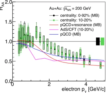
The transport coefficients are evaluated by several approaches of interactions be-tween heavy quarks and the medium including perturbative and non-perturbative QCD such as an interaction based on Ads/CFT correspondence, one taking into ac-count resonances of heavy and light quarks, or lattice QCD calculation [39, 40, 41, 42, 43]. Figure 2.15 shows RAA of electrons from heavy-quark decays in Au+Au with
√
s = 200 GeV [18], and theoretical estimations by several models [40, 41, 42]. The black and green points represent RAA of collisions with 0-92% and 10-20%
central-ities, respectively. The magenta line corresponds to the model based on AdS/CFT correspondence [41]. The blue line corresponds to the model based on pQCD [40]. The red line corresponds to the model based on pQCD including resonance states of heavy and light quarks in scattering amplitude. [40]. The red and blue lines show theoretical predictions for collisions with 0-92% centrality, and the magenta line show that for collisions with 10-20% centrality. The black and green boxes on RAA = 1
represents errors of Ncollfor black (0-92%) and green (10-20%) points, respectively. It
is hard to select the interaction models from the results of the heavy-quark electrons. It causes a large uncertainty of the spatial diffusion of heavy quarks, which related to η/s [36, 37, 44]. η/s values as a function of temperature of medium evaluated by several models are shown in Fig. 2.14 [36]. It is expected that the separation of charm and bottom are more informative to select them. Figure 2.16 shows RAAs
magenta line corresponds to the model based on AdS/CFT correspondence [41]. The blue line corresponds to the model based on pQCD [40]. The red line corresponds to the model based on pQCD including resonance states of heavy and light quarks in scattering amplitude. [40]. Solid and dashed lines represent RAAs of electrons from
charm and those from bottom, respectively. The red and blue lines show theoretical predictions for collisions with 0-92% centrality, and the magenta line show that for collisions with 10-20% centrality. Differences between each model are more clear than those in the results of electrons from heavy quarks without the separation.
Figure 2.14: η/s values as a function of temperature of medium evaluated by several
interaction models [36].
2.4
Separation of Charm and Bottom
2.4.1
Correlation of Decay Products
A fraction of bottom contribution in electrons from heavy-quark decays has been measured only for p+p collisions [15, 16]. They utilized correlations of electrons and hadrons from heavy quark decays to extract charm and bottom signals. Figure 2.17 shows the results of the measurements. The triangles and stars represent the results reported from PHENIX and STAR experiments, respectively. The associated squares and bars represent systematic and statistical errors, respectively. The bottom signal has been successfully extracted in p+p collisions.
Although this approach is succeeded for p+p collisions, it is hard to accomplish in A+A collisions due to a large combinatorial background due to a large amount
[GeV/c] T electron p 0 2 4 AA R 0.0 0.5 1.0 1.5 2.0 = 200 GeV NN s Au+Au: centrality: 0-92% (MB) centrality: 10-20% pQCD+resonance (MB) pQCD (MB) AdS/CFT (10-20%)
Figure 2.15: RAA of electrons from heavy-quark decays in Au+Au with
√
s = 200 GeV [18], and theoretical estimations by several models [40, 41, 42]. The
black and green points represent RAA of collisions with 0-92% and 10-20% centralities,
respectively. The magenta line corresponds to the model based on AdS/CFT correspon-dence [41]. The blue line corresponds to the model based on pQCD [40]. The red line corresponds to the model based on pQCD including resonance states of heavy and light quarks in scattering amplitude. [40]. The red and blue lines show theoretical predictions for collisions with 0-92% centrality, and the magenta line show that for collisions with
10-20% centrality. The black and green boxes on RAA = 1 represents errors of Ncoll for
[GeV/c] T electron p 1 2 3 4 5 AA R 0.0 0.5 1.0 1.5 2.0 = 200 GeV NN s Au+Au: pQCD+resonance (MB) pQCD (MB) AdS/CFT (10-20% cent.)
Figure 2.16: RAAs of electrons from charm and those from bottom for several interaction
models [40, 41, 42]. The magenta line corresponds to the model based on AdS/CFT cor-respondence [41]. The blue line corresponds to the model based on pQCD [40]. The red line corresponds to the model based on pQCD including resonance states of heavy and light
quarks in scattering amplitude. [40]. Solid and dashed lines represent RAAs of electrons
from charm and those from bottom, respectively. The red and blue lines show theoretical predictions for collisions with 0-92% centrality, and the magenta line show that for collisions with 10-20% centrality.
whereas, that in Au+Au collisions with √sN N = 200 GeV, dNchAA/dη|η=0= 242 ± 14
(687 ± 37) for centrality of 0-70% (0-5%) [46]. Therefore, the S/N ratio in Au+Au collisions is ∼1/100 smaller than that in p+p collisions due to increase of a com-binatorial background, and thus, statistical errors in Au+Au collisions increase to 10 times larger than those in p+p collisions. An alternative method is necessary to extract bottom signal in A+A collisions. The approach described in this thesis does not utilize a correlation, and is free from the combinatorial background. Therefore the approach is promising.
(GeV/c)
TElectron p
2
4
6
8
e)
→
e+b
→
e/(c
→b
0.0
0.2
0.4
0.6
0.8
1.0
PHENIX (correlation)
=200 GeV
s
p+p at
90% C.L.
90% C.L.
STAR (correlation)
Figure 2.17: The fraction of the bottom contribution in the heavy quark electrons as a
function of pT. The triangles and stars represent the results reported from PHENIX and
STAR experiments, respectively. The associated squares and bars represent systematic and statistical errors, respectively.
2.4.2
DCA Approach
Charm and bottom contributions in the electrons from heavy-quark decays are eval-uated by using DCA distributions in this thesis. The DCA depends on the life-times of the heavy-quark hadrons and q-values of their decay modes. Since life-times and q-values of charm hadrons and bottom hadrons are largely different, widths of their DCA distributions are also different, and thus, contributions of the charm and bot-tom electrons in the measured DCA distribution can be evaluated. Figure 2.18 shows
RMS values of DCA distributions of electrons from charm and bottom decays as a function of electron pT. The RMS values are calculated with a PYTHIA simulation.
Details of simulation tuning is described in Sec. 4.7.2. The black and red points represent RMS values for charm and bottom decays, respectively.
[GeV/c] T electron p 2 3 4 5 m] µ RMS [ 0 100 200 300 400 500
Figure 2.18: RMS values of DCA distributions of electrons from charm and bottom decays
as a function of electron pT. The black and red points represent RMS values for charm and
bottom decays, respectively.
A large difference of the DCA distributions of the electrons from charm and bottom is mainly derived from the difference of their life-times. The heavy-quark hadrons are decayed by the weak interaction. Most of the difference of the life-times is due to elements of the CKM matrix. The life-times and q-values for the decay modes with electron in their decay products are summarized in Table 2.1 and 2.2. Figure 2.19 shows examples of D meson and B meson decay diagrams accompanying an electron. The decay width (ΓHQ) can be written as
ΓHQ= mHQ 4 · (4π)3 & dxdyθ(x + y − xm)θ(xm− x − y + xy) ! |MHQ |2, (2.21)
where, x = 2Ee/mHQ and y = 2Eν/mHQ are the rescaled energies of electron and
neutrino in the heavy quark rest frame. xm = 1 − (mq/mHQ)2 is kinematic limit
to the energy transfer. As is shown in Eq. 2.6, the decay matrix elements are pro-portional to elements of the CKM matrix, and the corresponding elements for the charm and bottom decays are |Vcs| = 0.97344±0.00016 and |Vcb| = 0.0412+0.0011−0.0005,
Table 2.2: Life-times of charm and bottom hadrons. Hadron cτ D± 311.8 µm D0 122.9 µm Ds 149.9 µm Λc 59.9 µm B± 491.1 µm B0 457.2 µm Bs 441 µm Λb 417 µm c q s q W e ν + e b q c q W e ν -e