An optimal EOQ model for perishable products with varying demand pattern

An optimal EOQ model for perishable products with

varying demand pattern

Abdul, Ibraheem

1

_{and Atsuo Murata}

2

Department of Intelligent Mechanical Systems, Division of Industrial Innovation Sciences, Graduate School of Natural

Science and Technology, Okayama University, Okayama,

3-1-1, Tsushimanaka, Okayama, 700-8530 Japan.

1_{[email protected]}

2_{[email protected]}

Abstract — The demand pattern for most perishable products varies during their life cycle in the market. These variations must be properly reflected in inventory management in order to prevent unnecessary stock-out or excess inventory with associated increase in cost. In this paper, a multi-period economic order quantity (EOQ) model for managing the inventory of perishable items having varying demand pattern is presented. The model was formulated using a general ramp-type demand function that allows three-phase variation in demand pattern. These phases represent the growth, the steady and the decline phases commonly experienced by the demand for most products during their life cycle in the market. The model generates replenishment policies that guarantees optimal inventory cost for all the phases. Numerical experiments and sensitivity analysis were carried out to demonstrate the suitability of the model for a wide range of seasonal products. Result of the experiments revealed that the points at which demand pattern changes are critical points in managing inventory of products with ramp type demand.

I. INTRODUCTION

Perishable items are those items having a maximum usable lifetime e.g. foodstuff, human blood, photographic films, etc. Fresh produce, meats and other foodstuffs deteriorate gradually and become unusable after certain times. In drugs stores, medicines have fixed shelf lives while whole units of blood, photographic films are typical examples of items with limited useful life times. The maximum usable lifetime may be fixed, in which case the items become unusable at the end of a fixed period e.g. human blood. Lifetime for some products is assumed to be a random variable with its probability distribution represented by gamma, Weibull, exponential or any other distribution pattern. Due to its important connection with commonly used items in daily life, inventory modeling for perishable items continues to receive considerable attention among researchers.

Demand is a very important component of the inventory system, as the inventory problem will not exist without it. The nature of the demand determines the nature of model that will be developed to solve an inventory problem. The demand may be static or dynamic throughout the lifetime of the product or the system. Static demand are of rare occurrence in practice as demand for products often vary with several factors like time, price, stock etc. Some perishable products

are also seasonal in nature and demand for them exhibit various pattern during the season.

Ghare and Shrader [1] was the first to extend the classical EOQ formula to perishable items, wherein a constant fraction of on hand inventory is assumed lost due to deterioration. Subsequent works incorporated time varying demand patterns in modeling. Dave and Patel [2] developed the first perishable inventory model with dynamic demand in form of linear function of time. Sachan [3] and others improved Dave’s model by relaxing the no shortage assumption and assume complete backlogging of shortage and equal replenishment period. Later Hariga [4], Chang et al [5], and others introduced a general continuous log-concave demand function in place of the linear trend to cater for items with other forms of time dependent demand functions. However, the demand pattern in these models is unidirectional and not suitable for products whose demand pattern changes with time.

An Inventory model that caters for varying demand patterns was first proposed by Hill [6]. The model comprised a time dependent demand pattern that is a combination of two different types of demand in two successive time periods over the entire time horizon. This pattern, called ramp-type pattern, was observed by Wu [7] to be common in the case of new brand of consumer goods coming to the market. The demand rate for such items increases with time up to certain time and then ultimately stabilizes and becomes constant. Wu [7] developed a single-period EOQ model inventory for items that deteriorates at a Weibull rate, using ramp type demand rate.

The ramp type pattern was also found to be useful for seasonal products whose demand varies with the season. Thenceforth, several researchers have worked to develop inventory modeling for items having ramp type demand patterns. The works of Mandal and Pal [8], Wu [7], and Deng et al. [9] are notable contributions in this direction. Skouri et al [10] extended the frontiers of inventory models with ramp type demand by introducing a general ramp type demand pattern whose variable part is any positive function of time. All the ramp type models mentioned above, however, considered only a two-phase variation in demand patterns. This represents only the growth and the stable phases of demand.

Fifth International Workshop on Computational Intelligence & Applications

In real life, the demand for some products does not remain stable forever. It usually begins with increasing trend, attains a peak and becomes steady at the middle of its life cycle in the market, and finally decreases with time towards the end the cycle. This pattern is ramp-type in nature and has been observed to apply to many perishable items as well as seasonal items like fruits, fish, winter cosmetics, etc. (see Cheng and Wang [11]). Recently, Panda et al [12] observed that demand of seasonal products (fruits, e.g., mango, orange, etc., sea fish) over the entire time season is three folded. At the beginning of the season it increases, in the mid of the season it becomes steady and towards the end of the season it decreases and becomes asymptotic.

An inventory model for deteriorating seasonal products with three time periods classified as time dependent ramp-type function was developed by Panda et al [12]. Unlike previous ramp type models, this model allows a three-phase variation in demand patterns over time horizon. It however restricted the variation of demand during the growth and the decline phase to be of the same type. It also assumed that demand variation is an exponential function of time. These restrictions are not realistic in many inventory situations. The demand pattern during the growth and the decline phase may be different. Likewise the exponential increase/decrease in demand has been noted to be too high and may not be realistic in some real market situations.

In this paper, we develop a multi-period inventory model for perishable items using a general ramp-type pattern that allows three-phase variation in demand. The model relaxes previous unrealistic restrictions by allowing variations in demand patterns during the growth and the decline phase of demand. A general continuously increasing/decreasing function of time is used for the growth/decline phase of the ramp-type demand pattern to make the model suitable for different classes of perishable items with time dependent demand. The model seek to extend the works of Deng et al. [9] and others by considering three-phase variation in demand instead of two-phase variation that neglects the decline phase of demand. It also extends the model of Panda et al [12] by allowing variation in demand pattern during the growth and decline phase of demand. These are necessary extensions to enable the model suit some real life demand situations.

II. MODELASSUMPTIONSANDNOTATIONS

The following assumptions and notations are used in formulating the models:

1) A constant fraction ( θ

)

of on-hand inventory deteriorates per unit time.

2) Replenishment rate is infinite. 3) Shortages are not allowed.

4) No repair or replacement of deteriorated items during the period under review.

5) Inventory holding cost (H), replenishment cost (S), and cost of deteriorated items (P) are known and constant during the horizon.

6) The inventory level at any time (t) during the ith replenishment period is Ii(t)

7) The Length of the ith replenishment period and order quantity (Ti, and Qi

)

varies along the cycle.

8) The system has several replenishment periods during the horizon.

9) Demand rate f (t) is a general time dependent ramp-type function of the form:

( )

( )

( )

( )

( )

0,

( )

0, 0 ,

( ) ( )

. , . , , , 0 , b h a g b a t h t g b t t h b t a a g a t t g t f = ≤ ≤ ≥ ≥ ⎪ ⎩ ⎪ ⎨ ⎧ ≥ ≤ ≤ ≤ ≤ =

The function g(t) can be any continuously increasing function of time, while h(t) is any continuously decreasing function of time in the given interval. Parameters ‘a’ and ‘b’ represent the parameter of the ramp type demand function. The pattern f (t) is as depicted in Fig. 1.

f(t)

0 a b t Figure 1. The Ramp type demand pattern.

III. MODELFORMULATION

The inventory system consists several replenishment periods. Each period begins with full inventory and ends with zero inventory level. During the ith replenishment period, consumption due to demand and deterioration brings the inventory level to zero at the time Ti. Replenishment occurs at

time Ti and the cycle repeats itself. The objective is to

determine the replenishment schedules and order quantities (i.e. Ti, and Qi) for the first and all other subsequent periods

by minimizing the total inventory cost per unit time for each replenishment period. Fig. 2 shows a typical schedule.

Inventory level

0 1 3 time Figure 2. Variation of inventory level with time.

During a replenishment period the demand pattern will fall into any of the following categories:

1. Constant demand pattern: In this case demand pattern does not change during the period. The demand

function is a single function throughout the period. 2. Demand stabilization pattern: Demand pattern

changes from increasing to a constant pattern during the period. This is depicted in Fig. 2 at point ‘a’. 3. Declining demand pattern: Demand pattern changes

from constant pattern to declining pattern. This is depicted in Fig. 2 at point ‘b’.

4. Single period pattern: In this case both stabilization and decline of demand occurs during the same period. This is commonly encountered when a single replenishment is to be made to cover the entire horizon. The Demand pattern changes twice during the period.

The analysis of the system under these cases is considered below.

Case 1: Constant demand pattern.

The demand function, f (t), in this case may be a constant or an increasing/decreasing function of time. The equation of the inventory system for any replenishment period under this case is given by:

( )

_{( ) ( )}

. 0 , 0 i i i _{I t f t t T} dt t dI ≤ ≤ = + +θ (1) Since the inventory level is zero at time Ti, then Ii(Ti) = 0.

The solution to Eq. (1) above is given by Eq. (2) thus:

( )

t

(

tT x

( )

)

, 0 i.

i t e e f xdx t T

I ₌ −θ _∫i θ _{≤ ≤ (2)}

Total number of units in inventory during the ith replenishment period is given by I ₀TiI

( )

tdt,

i

I =∫ while total

number of units that deteriorate is given by I_D =θI_I.

The total inventory cost per unit time under this case (TC1i) is

given by:

(

)

1

(

(

)

)

. 1 1 I i I D i i S P H I T HI PI S T TC = + + = + θ+ (3)

Using Eq. (2) and the expression for II above in Eq. (3),

gives the general expression for the total inventory cost per unit time in this case.

(

)

(

(

( )

)

)

(

)

. 1 0 1 = + + ∫Ti −t∫tTi x i i _T S P H e e f xdx dt TC θ θ θ (4)

The first condition for minimizing total inventory cost per unit time (TC1i) is given by 1 =0.

i i dT

dTC _{Applying this}

condition to Eq. (4) above gives:

(

)

. 0 * 0 * H P S R dT dR T i i − = _θ+ (5)

( )

(

)

(

)

∫ − ∫ = Ti Ti t x t _{e f xdx dt} e R0 ₀ θ θ .

Solving Eq. (5) with the appropriate demand function gives the optimal length of the ith replenishment period, Ti*,

provided ₂1 0 2 > i i dT TC d

at the minimum point.

The optimal order quantity (Q1i*), obtained using Eq. (2), is:

( )

. * 0 * 1 e f tdt Q Ti t i=∫ θ (6)

Case 2: Demand stabilization pattern.

The equation of the inventory system in this case is as given below:

( )

_{( ) ( )}

( )

_{( ) ( )}

⎪ ⎪ ⎭ ⎪⎪ ⎬ ⎫ ≤ ≤ = + + ≤ ≤ = + + . , 0 , 0 , 0 i i i i i T t a a g t I dt t dI a t t g t I dt t dI θ θ (7)

Solution to Eq. (7) with the boundary condition Ii(Ti) = 0 and

Ii(a-) = Ii(a+) is given by:

( )

(

( )

( )

)

( )

(

( )

)

( )

_⎪ ⎭ ⎪ ⎬ ⎫ ≤ ≤ − = ≤ ≤ + = − − _{∫ ∫} . , 1 , 0 , i t T i T a x a t x t i T t a a g e t I a t dx a g e dx x g e e t I i i θ θ θ θ θ (8) The total number of units carried in inventory during the period is given in Eq. (9) below.

( )

( )

. 0I tdt I tdt I Ti a i a i I =∫ +∫ (9)

Total number of units that deteriorate is given by

ID =θII. (10)

The total inventory cost per unit time (TC2i ) is given by:

(

)

1

(

(

)

)

. 1 2 I i I D i i _T S PI HI _T S P H I TC = + + = + θ+ (11)

Substituting the expression for II in Eq. (11) followed by

some simplifications gives the expression for the total cost per unit time below.

(

)

(

)

( )

( )

(

)

(

)

(

)

. 1 0 2 2 ⎟ ⎟ ⎟ ⎟ ⎠ ⎞ ⎜ ⎜ ⎜ ⎜ ⎝ ⎛ + + ⎥ ⎥ ⎥ ⎦ ⎤ ⎢ ⎢ ⎢ ⎣ ⎡ _{− − − +} = ∫ − ∫ S H P dt dx x g e e a g a T e e T TC a a t x t i a T i i i θ θ θ θ θ θ θ (12)

Simplifying Eq. (12) and differentiating with respect to Ti

gives Eq. (13) below:

(

)

(

)

( )

(

(

)

)

{

/ 1

}

. 1 1 2 2 _{T P H e ga R P H S} T dT dTC T_i i i i i _{= + θ} θ _{− − θ+ + (13)}

( )

(

)

(

)

(

(

)

)

( )

₂ 0 1 θ θ θ θ θ θ _{e gxdx dt e e T a} ga e R =∫a −t ∫ta x + Ti− a− i− .

The necessary and sufficient condition for minimizing total inventory cost per unit time, TC2i , is 2 =0

i i dT dTC , provided 0 2 2 2 > i i dT TC d

at the minimum point. Applying this condition, using Eq. (13) gives:

(

/

)

1

( )

(

1

(

)

)

0. * * _{⎟ − + + =} ⎠ ⎞ ⎜ ⎝ ⎛ ₋ +H e ga R P H S P T Ti i θ θ θ (14)

Differentiating Eq. (13) with respect to Ti, and using the

first optimality condition stated in Eq. (14) above, we have

(

)

( )

. 1 * * 2 2 2 ⎥⎦ ⎤ ⎢⎣ ⎡ ₊ = P H e ga T dT TC d i T i i i _θ θ ₍₁₅₎

But g(a) > 0, and _eθTi* >0for all T

i. It therefore follows

from Eq. (15) above that ₂1 0

2 > i i dT TC d

. All conditions for a minimum value of TC2i are thus, satisfied and Eq. (14) gives

the optimal value of Ti*. The optimal order quantity, obtained

using Eq. (8), is shown below.

( )

*

( )

. 0 * 2 e gtdt e gadt Q Ti a t a t i=∫ θ +∫ θ (16)

Case 3: Declining demand pattern.

Demand pattern for the product changes from a constant value and begin to decrease with time during this phase. Equation of the system is represented in Eq. (17) below.

( )

_{( ) ( )}

( )

_{( ) ( )}

⎪ ⎪ ⎭ ⎪⎪ ⎬ ⎫ ≤ ≤ = + + ≤ ≤ = + + . , 0 , 0 , 0 i i i i i T t b t h t I dt t dI b t a g t I dt t dI θ θ (17)

The boundary conditions are Ii(Ti) = 0 and Ii(b-) = Ii(b+). The

solution to Eq. (17) is given by:

( )

(

( )

( )

)

( )

(

( )

)

_⎪⎭ ⎪ ⎬ ⎫ ≤ ≤ = ≤ ≤ + = ∫ ∫ ∫ − − . , , 0 , i T t x t i T b x b t x t i T t b dx x h e e t I b t dx x h e dx a g e e t I i i θ θ θ θ θ (18) The total number of units carried in inventory during the period is given in Eq. (19) below.

( )

( )

. 0I tdt I tdt I Ti b i b i I =∫ +∫ (19)

Using similar procedure as in case 2, the expression for the total cost per unit time is given below.

( )

( )

(

)

(

)

( )

(

)

(

)

(

)

. 1 0 3 ⎟ ⎟ ⎟ ⎠ ⎞ ⎜ ⎜ ⎜ ⎝ ⎛ + + ⎥ ⎥ ⎦ ⎤ ⎢ ⎢ ⎣ ⎡ + + = ∫ ∫ ∫ ∫ ∫ − − S H P dt dx x h e e dt dx x h e dx a g e e T TC i i i T b T t x t b b t T b x x t i i _{θ θ} θ θ θ θ (20) This expression is presented in a simplified form in Eq. (22).

If

(

(

( )

( )

)

)

( )

(

)

(

)

⎥⎥ ⎦ ⎤ ⎢ ⎢ ⎣ ⎡ + + = ∫ ∫ ∫ ∫ ∫ − − i i i T b T t x t b b t T b x x t dt dx x h e e dt dx x h e dx a g e e R θ θ θ θ θ 0 2 (21)

(

)

(

)

. 1 2 3 _T S P H R TC i i= + θ+ (22)

Applying the first condition for minimizing total inventory cost per unit time (TC3i ) to Eq. (22) gives:

(

)

. 2 * 2 * H P S R dT dR T i i − = _θ+ (23)

Solving Eq. (23) gives the optimal length of the ith

replenishment period (Ti*), provided ₂3 0

2 > i i dT TC d at the minimum point. The optimal order quantity (Q3i*), obtained

from Eq. (18) is as given below.

( )

*

( )

. 0 * 3 e gadt e htdt Q Ti b t b t i=∫ θ +∫ θ (24)

Case 4: Single period pattern.

This is when change in demand pattern occurs twice during a replenishment cycle. The equation of the system in this case is given by Eq. (25) below:

( )

_{( ) ( )}

( )

_{( ) ( )}

( )

_{( ) ( )}

⎪ ⎪ ⎪ ⎭ ⎪ ⎪ ⎪ ⎬ ⎫ ≤ ≤ = + + ≤ ≤ = + + ≤ ≤ = + + . , 0 , , 0 , 0 , 0 i i i i i i i T t b t h t I dt t dI b t a a g t I dt t dI a t t g t I dt t dI θ θ θ (25)

The solution to Eq. (25) with the boundary conditions;

Ii(Ti) = 0, Ii(b-) = Ii(b+), and Ii(a-) = Ii(a+) is given by:

( )

[

( )

]

( )

[

( )

]

( )

[

( )

]

⎪⎪_⎭ ⎪ ⎪ ⎬ ⎫ ≤ ≤ = ≤ ≤ + = ≤ ≤ + + = ∫ ∫ ∫ − − − . , , , , 0 , 1 2 1 i T t x t i b t x t i a t x t i T t b dx x h e e t I b t a F dx a g e e t I a t F F dx x g e e t I i θ θ θ θ θ θ (26) Where, ₁=_∫

( )

, ₂ =_∫b

( )

. a x T b exhxdx F e gadx F i θ θ

The total number of units carried in inventory during the period is given by:

( )

( )

( )

. 0I tdt I tdt I tdt I Ti b i b a i a i I =∫ +∫ +∫ (27)

The total inventory cost per unit time (TC4i ) is given by:

(

)

(

)

(

)

(

)

( )

(

)

(

)

. 1 5 4 1 0 1 2 3 4 ⎟ ⎟ ⎟ ⎟ ⎟ ⎠ ⎞ ⎜ ⎜ ⎜ ⎜ ⎜ ⎝ ⎛ + + ⎥ ⎥ ⎥ ⎥ ⎥ ⎦ ⎤ ⎢ ⎢ ⎢ ⎢ ⎢ ⎣ ⎡ + + + + + = ∫ ∫ ∫ − − − S H P dt F e dt F F e dt F F F e T TC i T b t b a t a t i i θ θ θ θ (28) Where 3=∫

( )

, 4 =∫

( )

, 5=∫tTi x

( )

. b t x a t exgxdx F e gadx F e hxdx F θ θ θ

As in Case 3 above, the expression in Eq. (28) can be simplified as shown in Eq. (29) below.

(

)

(

)

. 1 3 4 _T S P H R TC i i = + θ+ (29) Where,

(

)

(

)

(

)

(

)

( )

(

5

)

. 4 1 0 1 2 3 3 ⎥ ⎥ ⎥ ⎥ ⎥ ⎦ ⎤ ⎢ ⎢ ⎢ ⎢ ⎢ ⎣ ⎡ + + + + + = ∫ ∫ ∫ − − − i T b t b a t a t dt F e dt F F e dt F F F e R θ θ θ

Applying the first condition for minimizing total inventory cost per unit time (

TC

4i) to Eq. (29) gives:

(

)

. 3 * 3 * H P S R dT dR T i i − = _θ+ (30)

Solving Eq. (30) gives the optimal length of the ith replenishment period (Ti*), provided ₂4 0

2 > i i dT TC d at the minimum point. The optimal order quantity (Q4i*), obtained

from Eq. (26) is as given below.

( )

( )

*

( )

. 0 * 4 e gtdt e gadt e htdt Q Ti b t b a t a t i=∫ θ +∫ θ +∫ θ (31)

With the above equations, the optimal length of all replenishment periods and their corresponding cost and order quantities can be obtained throughout the horizon. A summary of the result is presented below:

(a). Replenishment period with no change in demand pattern:

Optimal length of period, Ti*, is given by Eq. (5).

Optimal inventory cost during period is TC1i* (Eq. (4)).

Optimal order quantity is Q1i* (Eq. (6)).

(b). Replenishment period with change in demand pattern (increasing to constant):

Optimal length of period, Ti*, is given by Eq. (14).

Optimal inventory cost during period is TC2i* (Eq. (12)).

Optimal order quantity is Q2i* (Eq. (16)).

(c). Replenishment period with change in demand pattern (constant to decreasing):

Optimal length of period, Ti*, is given by Eq. (23).

Optimal inventory cost during period is TC3i* (Eq. (22)).

Optimal order quantity is Q3i* (Eq. (24)).

(d). Replenishment period with double change in demand pattern (increasing - constant - decreasing):

Optimal length of period, Ti*, is given by Eq. (30).

Optimal inventory cost during period is TC4i* (Eq. (28)).

Optimal order quantity is Q4i* (Eq. (31)).

IV. SOLUTIONALGORITHM

To find the optimal replenishment schedules, costs, and order quantities over the entire time horizon, the following simple algorithm outline the procedure to follow. All replenishment periods are solved using the procedure for Case 1 except at the change points when demand pattern changes.

Step 1: Determine all the optimal values (Ti*, TC1i*, Q1i*) for

the first and subsequent replenishments using Eq. (5), Eq. (4) and Eq. (6) with appropriate demand function.

Step 2: Check for change points by comparing two successive values of t (i.e. ti and ti+1). (Note: ti+1 = ti + Ti, t0 = 0).

Step 3: If ti < a and a<ti+1≤b. Move a step backward and recalculate the optimal values (Ti*, TC2i*, Q2i*) for the period

using Eq. (14), Eq. (12) and Eq. (16).

Step 4: If a<ti≤b and ti+1 > b, Move a step backward and

recalculate the optimal values (Ti*, TC3i*, Q3i*) for the period

using Eq. (23), Eq. (22) and Eq. (24).

Step 5: If ti < a and ti+1 > b, Move a step backward and

recalculate the optimal values (Ti*, TC4i*, Q4i*) for the period

using Eq. (30), Eq. (28) and Eq. (31).

V. NUMERICALEXPERIMENTS

Two sets of experiments were conducted using numerical data to analyze the model behavior, and demonstrate its suitability for application to seasonal products. The numerical data for the experiments, presented below, were adapted from the models of Panda et al [12] and Cheng and Wang [11] involving perishable seasonal products.

Numerical data for Experiment 1:

( )

t Aexp

[

b

{

t

(

t μ

) ( ) (

H t,μ t γ

) ( )

H t,γ

}

]

. f = − − − − . 80 $ ; 300 ; 03 . 0 ; 3 ; 2 .

1 years = years = A= S= perorder

= γ θ μ . 01 . 0 ; 2 $ ; 10 $ = =

= perunit H perunit b P

( )

t,μ

H and H

( )

t,γ , are Heaviside functions. Numerical data for Experiment 2:

( )

⎪ ⎩ ⎪ ⎨ ⎧ ≤ ≤ − ≤ ≤ < + = . 112 112 , , 108 , , 4 100 2 2 1 1 t t t t t t f μ μ μ μ . 4 . 0 ; 4 ; 2 2 1= μ = θ= μ weeks weeks . 2 $ ; 3 $ ; 200

$ perorder P perunit H perunit

S= = =

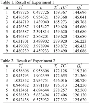
The demand functions, f (t), above represents single cases of the general ramp type model presented in this paper. The variable part of the general ramp function is represented by exponential function in experiment 1, and by a linear function in experiment 2. The numeric data were applied to the model one after the other, following the algorithm outlined earlier, and the result generated are shown in Table 1 and Table 2. Table 1. Result of Experiment 1

n Ti* ti Ti* .TCi* Qi* 1 0.477726 0.477726 159.367 144.696 2 0.476595 0.954321 159.368 145.041 3 0.484719 1.439040 165.273 149.768 4 0.476387 1.915427 159.620 145.680 5 0.476387 2.391814 159.620 145.680 6 0.476387 2.868201 159.620 145.680 7 0.631701 3.499902 279.920 156.223 8 0.479092 3.978994 159.872 145.433 9 0.480239 4.459233 159.490 145.086

Table 2. Result of Experiment 2

n Ti* ti Ti* .TCi* Qi* 1 0.958606 0.958606 172.128 119.210 2 0.943793 1.902399 172.655 121.360 3 1.032352 2.934751 456.016 150.720 4 0.946432 3.881183 176.313 124.250 5 0.813461 4.694644 278.257 92.560 6 0.938850 5.633494 177.406 126.120 7 0.942438 6.575932 177.332 125.620

VI. DISCUSSIONANDSENSITVITYANALYSIS Experiment 1 demonstrated the application of the model to perishable seasonal products with exponential ramp-type demand while experiment 2 shows the suitability of the model for products with trapezoidal demand. From the tables of result above, it can be observed that the values of optimal costs and order quantities for replenishment periods are generally close except at points where there is a change in demand pattern (e.g., n=3 and 7 in experiment 1, and n=3 and 5 in experiment 2 ). This shows that these points are critical points that must be well noted in managing inventory of perishable products with ramp type demand.

The result shown in Table 1 is the same with that obtained by Panda et al [12] when the time horizon is not fixed except at one of the change points (n=7). The difference in result at this point is believed to be due to a computational error on the part of Panda et al [12]. For further analysis of the model behavior, the result of a sensitivity analysis carried out based on the most critical replenishment period in the first experiment is shown in Table 3 below.

Table 3. Sensitivity analysis based on Experiment 1

Parameters % Change

in value of parameters

% Change in

Cost % Change in Order Quantity θ -25 -1.68 +7.87 -50 -3.33 +15.72 +25 +1.70 -7.91 +50 +3.44 -15.86 A -25 -10.73 -16.27 -50 -21.47 -33.79 +25 +10.73 +15.60 +50 +21.46 +30.78 P -25 -1.40 +1.23 -50 -2.80 +2.52 +25 +1.40 -1.16 +50 +2.80 -2.25 H -25 -9.33 +9.77 -50 -18.67 +25.55 +25 +9.33 -6.69 +50 +18.66 -11.58 S -25 -14.27 -9.47 -50 -28.54 -19.77 +25 +14.26 +8.82 +50 +28.53 +17.11 VII. CONCLUSION

The EOQ model developed in this paper generates optimal replenishment schedules and order quantity for perishable products having ramp type demand. The model extends the works of Deng et al. [9] and others by considering three-phase variation in demand instead of two-three-phase variation. It also extends the model of Panda et al [12] by allowing

variation in demand pattern during the growth and decline phase of demand.

Application of the model to perishable seasonal products with different demand patterns showed that it is suitable for a wide range perishable and seasonal products. The sensitivity analysis showed that the model is sensitive to changes in demand rate (A), inventory holding cost (H), and replenishment cost (S) while its sensitivity to deterioration rate (θ), and cost of deterioration (P) is low. This indicates, among other things, that the demand rate is an important factor in the model. It was also shown that the change points of demand pattern are critical points that must be well noted by managers in using the model.

Optimal replenishment policy generated by the model will assist inventory managers in ensuring minimum inventory costs for a wide range of perishable items. Consideration of shortages and partial backlogging of demand are recommended future works to further extend the application of the model.

REFERENCES

[1] P. M. Ghare, G. F. Schrader. A model for exponential decaying inventory, Journal of Industrial Engineering, Vol. 14, pp. 238-243, 1963. [2] U. Dave, L. K. Patel. (T, Si) policy inventory model for deteriorating items with time proportional demand, Journal of the Operational Research Society, Vol. 32, pp. 137–142, 1981.

[3] R. S. Sachan. On (T,Si) inventory policy model for deteriorating items with time proportional demand, Journal of the Operational Research Society, Vol. 35 (11), pp. 1013–1019, 1984.

[4] M. A. Hariga. Optimal EOQ model for deteriorating items with time-varying demand, Journal of the Operational Research Society, Vol. 47, pp. 1228-1246, 1996.

[5] H-J. Chang, J-T. Teng, L-Y. Ouyang, C-Y. Dye. Retailer's optimal pricing and lot-sizing policies for deteriorating items with partial backlogging, European Journal of Operational Research, Vol. 168, pp. 51–64, 2006.

[6] R. M. Hill. Inventory model for increasing demand followed by level demand, Journal of the Operational Research Society, Vol. 46, pp. 1250–1259, 1995.

[7] K-S. Wu. An EOQ inventory model for items with Weibull distribution deterioration, ramp type demand rate and partial backlogging, Production Planning and Control, Vol. 12 (8), pp. 787–793, 2001. [8] B, Mandal, A. K. Pal. Order level inventory system with ramp type

demand rate for deteriorating items, Journal of Interdisciplinary Mathematics, Vol. 1, pp. 49–66, 1998.

[9] P. S. Deng, R. H-J. Lin, P. Chu. A note on the inventory models for deteriorating items with ramp type demand rate, European Journal of Operational Research 2007, Vol. 178, pp. 112–120, 2007.

[10] K. Skouri, I. Konstantaras, S, Papachristos, I. Ganas. Inventory models with ramp type demand rate, partial backlogging and Weibull deterioration rate, European Journal of Operational Research, Vol. 192, pp. 79–92, 2009.

[11] M. Cheng, G. Wang. A note on the inventory model for deteriorating items with trapezoidal type demand rate, Computers and Industrial Engineering, Vol. 56, pp. 1296-1300, 2009.

[12] S. Panda, S. Senapati, M. Basu. Optimal replenishment policy for perishable seasonal products in a season with ramp-type time dependent demand, Computers and Industrial Engineering, Vol. 54, pp. 301–314, 2008.