九州大学応用力学研究所 Reports No.155(Sep. 2018)
18
0
0
全文
(2) CONTENTS. Analysis of the High Concentration of PM2.5 Observed in the Wide area of Japan in Late March 2018 by Using Chemical Transport Model By Yuki YAMAMURA, Itsushi UNO, Zhe WANG, Shunji NIIYA, Hisao CHIKARA, Syuhei NAKAGAWA………………………………………………………………...……………….….1. Numerical Simulation on Asymmetrical Interface of Floating Zone (FZ) for Silicon Crystal Growth By Xue-Feng HAN, Xin LIU, Satoshi NAKANO, Hirofumi HARADA, Yoshiji MIYAMURA and Koichi KAKIMOTO.……………………………….……………………………………………11.
(3) 九州大学応用力学研究所所報 第 155 号 ( 1 – 10 ) 2018 年 9 月. 2018 年 3 月下旬に国内広域で観測された高濃度 PM2.5 の 化学輸送モデルを用いた解析 山村 由貴*1, 2 鵜野 伊津志*3 王 哲*3 新谷 俊二*1 力 寿雄*1 中川 修平*1 (2018 年 8 月 10 日受理). Analysis of the High Concentration of PM2.5 Observed in the Wide area of Japan in Late March 2018 by Using Chemical Transport Model Yuki YAMAMURA, Itsushi UNO, Zhe WANG, Shunji NIIYA, Hisao CHIKARA, Syuhei NAKAGAWA E-mail of corresponding author: yamamura@fihes.pref.fukuoka.jp Abstract High PM2.5 concentration exceeding Japanese ambient criteria (daily mean 35μg/m3) were observed in late March 2018 over the wide area of Japan, and high PM2.5 concentration lasted for about a week. Aerosol observations and simulation by Chemical Transport Model illustrated the cause of this episode. In this episode, blocked high pressure existed over Japan, and it made subsidence inversion layer. Subsidence inversion layer suppressed the vertical diffusion, so pollutions were accumulated under this layer. Both particle SO42- and NO3- are transported from outside of Japan, but SO42- was mainly transported from China and NO3- was also from Korea. Simulated concentrations of PM2.5 well explained the time and space variation of observation data. But when effect of transboundary air pollution became high, simulated concentrations of PM 2.5 tended to be larger than observation, because anthropogenic emission data used was 2008 year base (REAS2008) and did not reflect recently decrease of Chinese emission. The model sensitivity analysis showed that SO42- was mainly transported from outside of Japan. NO3- concentration is effected by both the transboundary air pollution and local emission. For rural site like Oki, NO3- is mainly controlled by the transboundary air pollution, while for urban site like Osaka, local emission is more important than transboundary air pollution. Keywords: PM2.5, chemical transport model, transboundary air pollution, local pollution, sulfate, nitrate. 1.. し、2018 年 3 月下旬に、国内広域で PM 2.5 環境基準. はじめに. を超過し、さらに高濃度の大気汚染が 1 週間程度継. 微小粒子状物質 (PM 2.5 )は、健康影響が懸念さ. 続する現象が観測された。また、この事例では SO 4 2-. れることから、2009 年に大気環境基準(1年平均値. のみでなく、NO 3- も高濃度となっていたことが特徴. が 15μg/m3 以下であり、かつ、1日平均値が 35μg/m3. 的であった。本論文では、この広域・長期間におけ. 以下であること)が設定された。近年、中国におけ. る高濃度大気汚染現象について、エアロゾル化学成. る大気汚染物質の排出量の減少. 1) に伴い、日本国内. 分連続自動分析装置による PM 2.5 粒子成分分析結果、. の PM 2.5 濃度も減少している。一般大気環境測定局. および化学輸送モデルによるシミュレーション結. の環境基準達成率は、2014 年から 2016 年にかけて、. 果から、その原因を明らかにした。. 関東は 34.6%から 97.4%、東海は 25.9%から 98.7%、 近畿は 61.1%から 95.3%、中国は 14.0%から 75.8%、 四国は 31.0%から 66.7%、九州は 6.8%から 61.5% となり、いずれの地域でも改善がみられた 2) 。しか *1 *2 *3. 福岡県保健環境研究所 九州大学大学院総合理工学府 九州大学応用力学研究所. 2.. 方法. 2.1. PM 2.5 成分濃度測定. 観測データには、九州大学 応 用力学研究 所 屋上に 設置 した、エアロゾル化学 成分 連 続 自動 分 析 装置 (Continuous Dichotomous Aerosol Chemical Speciation.
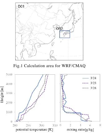
(4) 山村・鵜野ほか:2018 年 3 月下旬に国内広域で観測された高濃度 PM2.5 の化学輸送モデルを用いた解析. Analyzer,ACSA-12;紀本電子工業製)で測定された 1 時間毎の硫酸塩(SO 4 2- )濃度、硝酸塩(NO 3- )濃度およ び太宰府局(福岡県)、国設 大阪(大阪府)、国設隠岐 (島根県)に設置された常時監視局 PM 2.5 濃度の速報 値を使用した。ACSA-12 の測定は紀本ら. 3) に準じて行. われた。. 2.2. 化学輸送モデル. 気 象 場 の 計 算 に は 、 領 域 気 象 モ デ ル Weather Research. and. Forecasting. 3.9.1.1 4) を使用した。WRF. model. (WRF). Fig.1 Calculation area for WRF/CMAQ. version. の初期条件および境界条件. には、米 国 環 境 予 報 センター (NCEP) の全 球 客 観 解 析データ (FNL) 5) を使用した。計算領域 は、東アジア 域 (D01、64km 格子) および西日本域 (D02、16 km 格 子 ) の二 重 格 子 とした。鉛 直 層は、地 表 面 から上 空 100hPa までを 29 層に分割した。地形データセットには、 United States Geological Survey (USGS) の全球数値 標高データを用いた。 汚染物質濃度の計算には、化学輸送モデル CMAQ version 5.0.2 6)7) を使用した。大気中の汚染物質および その前 駆物 質の反 応過 程として、気相 化学 反 応に. Fig. 2 Potential temperature and water vapor mixing. SAPRC07、エアロゾル過程に AERO6 を使用した。排出. ratio at Fukuoka District Meteorological Observatory. 量データには、東アジア域における人為起源排出量は Regional Emission inventory in Asia (REAS) version. 3 月 24 日から 30 日は、日本東岸でジェット気流が蛇行・. 2 8) を、中国の NH. 収束しため、高気圧の東進が妨げられ、長期間西日本、. 3 排出量について Streets. et. al. 9) に基づ. き排出量の季節変動を補正して使用した。船舶起源排. 東日本が広く帯状の高気圧に覆われていた 16) 。24 日か. 出量は海洋政策研究財団 (OPRF) が作成した船舶排. ら 26 日 9:00 に福岡管区気象台で観測された温位およ. 10) を使用した。日本域における人為起源. び水蒸気混合比のエマグラムを Fig.2 に示す。Fig.2 か. 排 出源 のうち、自 動 車 起 源のものは JATOP Emission. ら、24 日は 1000m、25 日は 800m、1500m、26 日は. Inventory-Data. 出インベントリ. Source. 200m、800m 付近に逆転層が確認できた。混合比は逆. (JEI-DB2011-AS) 11) 、自動 車・船舶 以 外の人 為起 源 排. 転 層 底 部 から上 部 にかけて急 激 に低 下 し、逆 転 層 より. 出源は、EAGrid2010-Japan 12) を使用した。植生起源排. 上層で低くなっていた。これより、高気圧性の下降気 流. 出量は Model of Emissions of Gases and Aerosols from. による沈降性逆転層が生成していたと考えられる。. Base. 2011. Automobile. version2.04 により推計した。火山. 24 日から 26 日のモデル(D01)による PM 2.5 濃度の. 起源の SO 2 排出量は Aerosol Comparisons between. 12 時間毎の水平分布を Fig.3 に示す。PM 2.5 について. Observations and Models (AeroCom) によって作成され. は、24 日 15:00 には九州の西に位置する高気圧の影響. たデータ 14) を使用し、国内の浅間山、御嶽山、三宅島、. により、中国 北東 部 の高 濃度 汚染 気塊が東へ移流し、. 阿 蘇 山 、桜 島 、口 之 永 良 部 島 については気 象 庁 の火. 日本にも流入していた。25 日 3:00、15:00 には、西日本. Nature. (MEGAN) 13). 山活動解説資料. 15) の. を中心に韓国からも汚染気塊が流入した。26 日 3:00 に. SO2 排出量を使用した。. は、北海 道 の西 に位置する低 気 圧の影 響が強まり、日. WRF/CMAQ の 計 算 領 域 を Fig.1 に 示 す 。. 本への汚染気塊の流入が減少した。. WRF/CMAQ の計算期間は 3 月 1 日から 4 月 10 日とし、. 24 日から 26 日のモデル(D01)による O3 および微小. 3 月 23 日から 31 日を解析対象期間とした。. 粒子状 SO 4 2- 、NO 3- 濃度の 12 時間毎の水平分布をそれ. 3.. 結果と議論. 3.1. PM 2.5 濃度と気象状況. ぞれ Figs.4、5、6 に示す。SO 4 2- 、NO 3 - 共に西よりの風に よって国外から輸送されているが、SO 4 2- は中国からの影 響が大きく、NO 3 - は韓 国からの影 響 も大 きいことが判っ た。. 2.
(5) 山村・鵜野ほか:2018 年 3 月下旬に国内広域で観測された高濃度 PM2.5 の化学輸送モデルを用いた解析. Fig.3 Modeled PM 2.5 concentration for Domain D01.. Fig.4 Modeled O 3 concentration for Domain D01.. 3.
(6) 山村・鵜野ほか:2018 年 3 月下旬に国内広域で観測された高濃度 PM2.5 の化学輸送モデルを用いた解析. Fig.5 Modeled NO 3 - concentration for Domain D01.. Fig.6 Modeled SO 4 2- concentration for Domain D01.. 4.
(7) 山村・鵜野ほか:2018 年 3 月下旬に国内広域で観測された高濃度 PM2.5 の化学輸送モデルを用いた解析. Fig.7 Modeled O 3 concentration for Domain D02.. Fig.8 Modeled NO 3 - + HNO 3 concentration for Domain D02.. 5.
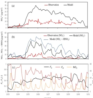
(8) 山村・鵜野ほか:2018 年 3 月下旬に国内広域で観測された高濃度 PM2.5 の化学輸送モデルを用いた解析. Fig.9 Modeled SO 4 2- concentration for Domain D02. O 3 については、24 日 15:00 に中国大陸で高濃度とな. る。. り、25 日夜間 3:00 は NO による分解の影響が少ない海 上で高濃度を維持し、25 日 15:00 には中国大陸で再び 高濃度となり、海上に残っていた O 3 と共に、朝鮮半島、 日本へ流入した。この時、NO の一次排出源付近では、 O 3 + NO → NO 2 + O2. (1). によって O 3 が消費されるため、韓国等の陸上では O 3 濃 度が低くなっていたと考えられる。それぞれの成分の濃 度分布について、D02 での水平分布を用いて、詳細に. (2). NO 3 + NO 2 + M ⇄ N2 O 5 + M. (3). N 2 O5 + H 2 O → 2HNO 3. (4). NO 3 + RCHO → HNO 3 + RCO. (5). 一方、15:00 の NO 3- +HNO 3 の高濃度領域は、それま. 比較する。. でに比べ減少していた。HNO 3 の海面への沈着により、. 24 日から 25 日のモデル(D02)による O 3 、微小粒子. 濃度が減少した可能性も考えられる。. 状 NO 3 - と HNO3 濃度の和(NO 3- +HNO 3)、微小粒子 状 SO 4. O 3 + NO 2 → NO3 + O 2. 一方、SO 42- は昼夜共に O 3 高濃度領域で高濃度とな. 2- 濃度の 6 時間毎の水平分布をそれぞれ Figs.7、. っており、さらに海上を吹走中に濃度が増加していた。. 8、9 に示す。O 3 の高濃度領域と NO 3- +HNO 3 の高濃度 領 域 を比 較すると、夜 間 から朝 にかけて(3:00, 21:00,. 3.2. 9:00)は、NO 3- +HNO 3 が高濃度となった領域で O 3 濃度. 福岡における PM 2.5 濃度上昇要因の解析. は低くなり、日中(15:00)は、NO 3- +HNO3 と O3 の高濃度. ACSA による SO 42- 、NO 3- 濃度の時間変化とモデルに. 領域がほぼ一致していた。夜間においては、以下のよう. よる計算結果を合わせて Fig.10(a)、(b)に示す。濃度の. な O3 による酸化が NO 3 - 、HNO3 の生成に大きく寄与し. 増減傾向は ACSA とモデルで類似しており、ACSA、モ. た. O 3 の生成が盛んな日中と異なり、夜間. デル共に、24 日から 26 日にかけて SO 4 2- 、NO 3- 濃度が. は O 3 が NO、NO 2 の酸化に使用されることで減少し、. 高まっていた。しかし、濃度の値は ACSA に比べ、モデ. NO 3- 、HNO 3 は酸化により生成するため、NO 3- +HNO 3 が. ルが大きく、越境汚染の影響の大きかった 24 日から 30. 高濃度となった領域で O 3 濃度が低くなったと考えられ. 日にかけて特に過大評価となっていた。これはモデルで. 17) 、すなわち. 6.
(9) fNO3. fNO3. 45 45 40 40 35 35 30 30 25 25 20 20 15 15 10 10 5 5 0 0 fSO4fNO3 fNO3 3/14 fNO3 3/10 3/11 3/123/10 3/133/11 3/143/12 3/153/13 3/16 3/173/15 3/183/16 3/193/17 3/203/18 3/213/19 3/223/20 3/233/21 3/243/22 3/253/23 3/263/24 3/273/25 3/283/26 3/293/27 3/303/28 3/313/29 3/30 3/31 40 45 45 Observation Model 60 ACSA CMAQ ACSA CMAQ 35 40 (a) 40 35 30 35 50 30 25 30 40 25 20 25 20 20 15 30 15 15 10 10 10 20 1 0.05 0.05 1 0.05 5 1 5 5 0 0 10 0 fNO3 3/23 3/25 3/26 3/27 3/28 3/29 3/30 3/31 0.8 0.8 0.04 3/10 3/11 3/12 3/13 3/14 3/15 3/16 3/17 3/18 3/19 3/20 3/213/26 3/223/27 3/233/28 3/24 3/25 3/263/31 3/27 3/280.04 3/29 3/30 3/31 0.8 3/10 3/11 3/24 3/12 3/13 3/14 3/15 3/16 3/17 3/18 3/19 3/20 3/21 3/22 3/23 3/24 3/25 3/29 3/30 S 0.04 0 60 ACSA3/23 3/24 CMAQ -) ACSA 3/10 3/11 3/12 3/13 3/14 3/15 3/16 3/17 3/18 3/19 3/20 3/21 3/22 3/25 3/26 3/27 3/28 3/29 3/30 3/31 Observation (NO CMAQ ACSA CMAQ Model (NO3 ) 3 50 0.6 (b) 0.6 0.03 0.03. 山村・鵜野ほか:2018 年 3 月下旬に国内広域で観測された高濃度 PM2.5 の化学輸送モデルを用いた解析. 0.6ACSA. 40 30 0.4 20. 0.2. 10 0 0 3/23 3/24 1. 0.8 FS, FN [-]. 𝐹𝑁 =. [𝑆𝑂42− ] [𝑆𝑂2 ] + [𝑆𝑂42− ]. (6). [𝑁𝑂3− ] [𝐻𝑁𝑂3 ] + [𝑁𝑂3− ]. (7). F は 26 日付近から、緩やかに増加している。越境汚染. (c). CMAQ. Model (NO3 TNO3. - + HNO ) 3. により流入する SO 2 が減少し、さらにそれまでに蓄積さ れていた SO2 も、時間の経過と共に酸化され、SO 4 2- を生 0.02. 0.4. 0.4. 0.02. 0.02. 0.2. 0.2. 0.01. 0.01. がみられた。これは、26 日付近から越境汚染により粒子. 0. 0. 0. 0. 0 として流入する NO 3- が減少したためと考えられる。なお、 3/30. 3/24 3/25 3/25 3/26 3/25 3/27 3/27 3/28 3/31 3/29 3/30 3/25 3/26 3/28 3/26 3/27 3/29 3/293/27 3/283/30 3/303/28 3/29 3/24 3/263/24 40 ACSA CMAQ TNO3 SO4/(SO2+SO4) (HNO3+NO3)/(NO2+HNO3+NO3) NO2 SO4/(SO2+SO4) (HNO3+NO3)/(NO2+HNO3+NO3) NO2 SO4/(SO2+SO4) (HNO3+NO3)/(NO2+HNO3+NO3) NO2 FS FN NO 2. 30. 0.6 20 0.4. 3/24. 3/25. 3/26 SO4/(SO2+SO4). 3/27. 3/28. NO3/(HNO3+NO3) MM/DD. 3/29. 3/30. 成したためと考えられる。F N は、26 日付近から減少傾向 0.01. いずれの日においても 7:00、18:00 付近で F N 、NO 2 が極 大となっていた。7:00、18:00 は通勤時間帯であることか ら、近傍の道路交通量の増加による NO 2 排出量の増加 を反映したためと考えられる。. 10. 0.2 0 3/23. 0.03. NO2 [ppb]. NO3-, NO3- + HNO3[μg/m3]. SO42- [μg/m3]. 𝐹𝑠 =. 太宰府市(福岡)の CMAQ での PM 2.5 濃度および温. 0 3/31. 位の鉛直分布を Fig.11 に示す。Fig.11 から、高気圧性. NO2. の下降気流により断熱昇温が起きていることが確認でき Fig.10 Observed and modeled concentration of (a). た。また、特 に 高 濃 度 となっ た 25、26 日 は、どち らも. SO 4 2- , (b) NO3 - , NO 3- + HNO 3, (c) modeled FS , F N and. Fig.2 のエマグラム中の逆転層位置である高度約 800m. NO 2 concentration. 以下の濃度が上 昇していた。これは沈降性逆 転層によ って鉛直方向の拡散が抑制されたことで、逆転層より下 層に汚染が蓄積したと考えられる。 以上から、国外からの汚染気塊の流入が減少した 26 日以降は、SO 4 2- については(NH 4) 2 SO4 等の硫酸塩粒 子として滞留し続けたため、長期間高濃度が持続したと 考えられる。一方 NO 3 - は SO 4 2- と異なり、NH 4 NO 3 として 流入しても、温度の上昇に伴いガスへ分解されるため、 SO 4 2- のように長期間滞留することができず、国外からの 流 入 の減 少 と共 に、濃 度 が急 激 に減 少 したと考 えられ る。. 3.3. Fig. 11 Modeled PM 2.5 concentration and potential temperature profile at Dazaifu. 各地域の PM 2.5 濃度変化とモデルの再現性. 太宰府市(福岡)、隠岐の島町(島根)、大阪市(大阪) におけるモデルと常時監視局の PM 2.5 濃度時間変化を Fig.12 に 示 す 。 図 中 に は 、 デ ー タ 数 (N) 、 Mean. は中国の排出量データに REAS2008 を使用しており、. Fractional Bias. 近年の中国の大幅な排出量削減を反映できていないこ. (MFB). と Mean Fractional Error. (MFE) を示している。MFB と MFE は、以下の計算式に. とが原因と考えられた。また、ACSA、モデル共に、国外. より求めた。. からの高濃度汚染気塊の流入が減少した 26 日から、 NO 3- 濃度が大きく減少していた。一方、SO 4 2- 濃度は 26. 𝑁. 日以降緩やかに減少しているが、30 日付近まで高濃度. 𝑀𝐹𝐵 =. が継続していた。. 2 (𝑀𝑖 − 𝑂𝑖 ) ∑ × 100 𝑁 (𝑀𝑖 + 𝑂𝑖 ). (8). 𝑖=1. ここで、以下で定義される F S 、FN および NO2 濃度の. 𝑁. 太宰府における時間変化を Fig.10(c)に示す。. 𝑀𝐹𝐸 =. FS 、F N は 0 から 1 の値を取り、F S は SO 2 の粒子化が、. 2 | 𝑀𝑖 − 𝑂𝑖 | ∑ × 100 𝑁 (𝑀𝑖 + 𝑂𝑖 ) 𝑖=1. F N は NO2 の粒子化が進むほど値は大きくなる。. 7. (9).
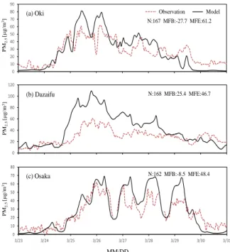
(10) Osaka_PM2.5 Osaka_PM2.5 80. 80. 70. 70. 60. 60. 50. 50. 40 40 山村・鵜野ほか:2018 年 3 月下旬に国内広域で観測された高濃度 PM2.5 の化学輸送モデルを用いた解析 30 30. PM2.5 [μg/m3]. 70. 20. 10. 10. Oki_PM2.5 0 0 3/10 3/11 3/103/12 3/113/13 3/123/14 3/133/15 3/143/16 3/153/17 3/163/18 3/173/19 3/183/20 3/193/21 3/203/22 3/213/23 3/223/24 3/233/25 3/243/26 3/253/27 3/263/28 3/273/29 3/283/30 3/293/31 3/30 3/31. 地域的な発生源の感度解析を行った。. 90. 80. 20. Observesion Observesion Observation. (a) Oki. 太 宰 府 市 (福 岡 )、隠 岐 の島 町 (島 根 )、大 阪 市 (大. CMAQ CMAQ Model. N:167 MFB:-27.7 MFE:61.2. 阪)の SO 42- 、NO 3- 濃度の CNTL および JPEM0 を Fig.13. 60. 50. に示す。太宰 府、大 阪は共に都市 部であるが、太 宰府. 40 30. はより越境汚染の影響を受けやすく、大阪はより地域発. 20 10 0 3/23 120. PM2.5 [μg/m3]. 100. 3/24. 3/25. 3/26 Fukuoka_PM2.5 3/27 Observesion. 3/28. 3/29. 3/30. 生源からの排出量が多い特徴を持つ。一方、隠岐は地. 3/31. 域 発 生 源 の 少 な い 地 域 で あ る 。 SO 42- に つ い て は 、. CMAQ. N:168 MFB:25.4 MFE:46.7. (b) Dazaifu. CNTL、JPEM0 共にいずれの地域も幅の広いピーク形. 80 60. 状をしていた。また、いずれの地域においても CNTL と. 40. JPEM0 の濃度差は小さく、越境汚染の影響が大きいこ. 20 0 3/23. とが示唆された。 3/24. 3/25. 3/26. 80. PM2.5 [μg/m3]. 70. Osaka_PM2.5 3/27 Observesion. 3/28. 3/29. 3/30. NO 3- は、太宰府、大阪においては、CNTL は日内変. 3/31. CMAQ. 動による鋭いピークが見られ、日中と夜間の濃度差は太. N:162 MFB:-8.5 MFE:48.4. (c) Osaka. 60. 宰府に比較して、大阪で大きくなっていた。JPEM0 は、. 50 40. 隠岐では CNTL との差は無く、ほぼ越境汚染の影響で. 30 20. あることが示された。太宰府では 24 日夕方から 26 日夜. 10 0 3/23. 3/24. 3/25. 3/26. 3/27 Observesion. MM/DD. 3/28. 3/29. 3/30. 間までは CNTL との濃度差は小さく、越境汚染の影響. 3/31. が大 きいことが示された。また、越 境 汚 染 によって粒 子. CMAQ. Fig. 12 Observed and modeled PM 2.5 concentration for. 状の NO 3- が流入することから、この期間は特に日中もベ. (a) Oki, (b) Dazaifu, (c) Osaka. ースが高くなる傾向が確認された。一方 、大阪では、太 宰府・隠岐に比べて CNTL と JPEM0 の濃度差が大きく、 地域汚 染の影 響が大きいことが示 された。さらに、隠岐、. ここで、i は時間、Mi は i 時におけるモデルの計算値、. 太宰府に比べて日中と夜間の濃度差が顕著 であった。. Oi は i 時における実測値、N はデータ数を示す。この定. NO 3- +HNO3 で評価すると、日中の濃度は NO 3 - のみに. 義により MFB は–200%~+200%,MFE は 0%~+200%. 比べて増加していることから、温度上昇により、NH 4 NO 3. の範囲の値をとる。MFB と MFE は、モデルを科学的知. の平 衡が気 相 側にシフトし、HNO 3 が増加したことが示. 見の拡充や規制対策などに十分適用可能な. 唆された。しかし、NO 3 - +HNO 3 においても、夜間に比べ. performance goal (MFB≦±30%,MFE≦+50%) と、そ. ると日中の濃度は大きく減少しており、HNO 3 の沈着等. れ ら へ の 適 用 が 妥 当 と み な せ る performance criteria. が起きた可能性が考えられた。. (MFB≦±60%,MFE≦+75%) が提唱されている. 18) 。. PM 2.5 中 の NO3- 濃 度 は SO 4 2- と 同 様 に 高 いた め、. 24 日から 30 日の太宰府、大阪の MFB はそれぞれ. NO 3- 濃度の日内変動を反映し、Fig.12(c)で示された大. 25.4%、–8.5%、MFE はそれぞれ 46.7%、48.4%であり、. 阪の PM 2.5 濃度の鋭いピークができたと考えられた。. performance goal を満たしていた。また、隠岐の MFB、. SO 4 2- がいずれの地 域 においても越 境 汚 染の影 響が大. MFE は–27.7%、61.2%であり、performance criteria を満. きいのに対し、NO 3 - は地 域の特 徴によって寄 与 率が異. たしていた。隠 岐 、太 宰 府 において、越 境 汚 染 の影 響. なり、都心部では地域汚染の寄与率が高く、さらに九州. が特に大きいと考えられる 24 日から 29 日に過大評価傾. から西 日 本の地 域のほうが越 境 汚 染の影 響 が大 きくな. 向が見られたが、これは 3.2 の ACSA との比較で述べた. る傾向が確認された。. REAS2008 の影響と考えられる。 Fig.12 では、いずれの地域においても、モデル・観測. 4.. 共に PM 2.5 濃度は 24 日から 30 日付近で高まっている. ま と め. が、太 宰 府 ・隠 岐 がベースの高 い幅 の広 いピーク形 状. 2018 年 3 月下旬に、国内広域で PM 2.5 環境基準を. であるのに対し、大阪では日中濃度が低 下し夜間に上. 超過し、高濃度の大気汚染が 1 週間程度継続する現象. 昇する日内変動による鋭いピークが顕著であった。この. が観 測された。本 論 文 では、エアロゾル化 学 成 分 連 続. 原 因 に つ いて 、 感 度 解 析 を 用 いて 次 節 で 検 証 す る。. 自動分析装置および化学輸送モデルを用いて、その原. 3.4. 因を考察した。. 国内汚染寄与率の地域変化. 高濃度となった 3 月 24 日から 30 日は、日本東岸で. 全 ての排 出 量 を含 む設 定 (CNTL)と国 内 の人 為 起. ジェット気流が蛇 行・収束したことで高気圧の東 進が妨. 源排出量を 100%削減した設定(JPEM0)で計算を行い、. げられ、長期間西日本、東日本が広く帯状の高気圧に. 8.
(11) 山村・鵜野ほか:2018 年 3 月下旬に国内広域で観測された高濃度 PM2.5 の化学輸送モデルを用いた解析 24 日夕方から 26 日夜間まで越境汚染の影響が大きく、 大阪では、太宰府・隠岐に比べて地域汚染の影響が大 きいことが示唆された。. 謝辞 排 出 量 データの作 成 は、大 阪 大 学 大 学 院 工 学 研 究 科 嶋 寺 光助 教からプログラムをご提 供 いただきました。 また、電 力 中 央 研 究 所 の板 橋 秀 一 主 任 研 究 員 には、 CMAQ の感度解析のサポートを受けました。ここに記し て謝意を表します。. 参考文献 1). Fu, X., Wang, S., Xing, J., Zhang, X., Wang, T., Gao, J.: Increasing ammonia concentrations reduce the effectiveness of particle pollution control achieved via SO2 and NOX emissions reduction in East. China,. Environ.. Sci.. Tech.. Lett.,. doi:10.1021/acs.estlett.7b00143 , 2017. 2). 鵜 野 伊 津 志,王 哲,弓 本 桂 也,板 橋 秀一,長 田 和 雄,入 江 仁 士,山 本 重 一,早 崎 将光,菅. Fig. 13 Fig.13 Modeled concentration of SO 4 2- , NO 3-. 田 誠治:PM2.5越境 問題は終焉に向かっているの. for (a) Oki, (b) Dazaifu, (c) Osaka, and NO 3- + HNO 3. か?, 大気環境学会誌,52,177-184, 2017.. for (d) Osaka. 3). 紀本英志、植田明子、辻本賢太、三谷洋一、戸 矢崎保雄、紀本岳志 : 大気エアロゾル化学成分 連続自動分析装置の開発, クリーンテクノロジ. 覆 われていた。高 気 圧 により沈 降 性 逆 転 層 が発 生 し、. ー, 23, 49-52, 2013.. 鉛直方向の拡散が抑制されたことで、逆転層より下層に. 4). 汚染が蓄積しやすい状態となっていた。. Skamarock, W.C., Klemp, J.B., Dudhia, J., Gill, D. D., Barker, D. M., Duda, M. G., Huang,. SO 4 2- 、NO 3- 共 に西 よりの風 によって国 外 から輸 送 さ. Wang,. W.,. X.-Y.,. Powers, J. G.: A Description of the. れており、越境の影響が強かった 24 日から 26 日にかけ. Advanced Research WRF Version 3, NCAR Tech.. て、特に濃度が高くなっていた。SO 42- は中国からの影響. Note, NCAR/TN-475+STR, 113 pp., Natl. Cent.. が大きく、NO 3. - は韓国からの影響も大きかった。. for Atmos. Res., Boulder, Colorado, USA , 2008.. O3 と NO3 - +HNO3 の濃度分布は、夜間から朝にかけ ては NO 3. - +HNO. 3. 5). が高濃度となった領域で O 3 濃度は低. Data. Archive,. クセス).. 一 致していた。このことから、NO、NO 2 の酸 化には、夜. 6). 間は O 3 、日中は OH 等他の物質が主に寄与しているこ とが示唆された。一方 SO 4. Research. http://rda.ucar.edu/datasets/ds083.2/ (2018.7.11 ア. くなり、日中は、NO3 - +HNO 3 と O 3 の高濃度領域がほぼ. 2- は、昼夜共に. CISL:. Byun D, Ching J: Science algorithms of the EPA Models-3. O 3 高濃度領. (CMAQ). 域で高濃度となっており、さらに海上を吹走中に濃度が. Community. Multiscale. Air. modeling. Quality system.. EPA/600/R-99/030 ,1999.. 増加していた。. 7). Byun D, Schere KL: Review of the governing. 太 宰 府 、隠 岐 、大 阪 において、全 ての排 出 量 を含 む. equations, computational algorithms, and other. 設定と国内の人為起源排出量を 100%削減した設定で. components of the models-3 Community Multiscale. 感度解析を行った。その結果、SO 4 2- と NO3 - の主な発生. Air Quality (CMAQ) modeling system. Applied. 源が、地域の特徴によって異なることが判った。SO 4. 2- に. Mechanics Reviews, 59(1-6), 51-76. ,2006.. ついてはいずれの地域においても越境汚染の影響が大 きいことが示唆された。一方 NO 3. 8). - は、太宰府・隠岐では. Ohara, T., Akimoto, H., Kurokawa, J., Horii, N., Yamaji, K., Yan, X., and Hayasaka, T:An Asian. 9.
(12) 山村・鵜野ほか:2018 年 3 月下旬に国内広域で観測された高濃度 PM2.5 の化学輸送モデルを用いた解析. emission. inventory of anthropogenic emission. Nature), Atmos. Chem. Phys., 6, 3181–3210, 2006.. sources for the period 1980–2020.Atmos. Chem. 9). 14) Diehl T., Heil A., Chin M., Pan X., Streets D.,. Phys., 7, 4419-4444, 2007.. Schultz, M., Kinne, S.: Anthropogenic, biomass. Streets D.G., Yarber K.F., Woo J.-H., Carmichael. burning, and volcanic emissions of black carbon,. G.R. Biomass burning in Asia: Annual and seasonal. organic carbon, and SO2 from 1980 to 2010 for. estimates. hindcast model experiments, Atmos. Chem. Phys.. and. atmospheric. emissions.. Global. Biogeochemical Cycles, 17(4), 10/1-10/20, 2003.. Discuss., 12, 24895–24954, 2012.. 10) 海洋政策研究財団 : 平成22年度 排出規制海域. 15) 気 象 庁 : 火 山 解 説 資 料 (2018),. 設定 による大気 環 境 改善 効 果の算定 事 業 報告 書 ,. https://www.data.jma.go.jp/svd/vois/data/tokyo/ST. ISBN978-4-88404-265-3, 2010.. OCK/monthly_v-act_doc/monthly_vact.php(2018.7.. 11) (一 財 )石 油 エネルギー技 術 センター:JATOP 技 術. 30アクセス).. 報告書「自動車排出量推計」, JPEC-2011AQ-02-06,. 16) 鵜野 伊津志、山村 由貴、王 哲: 越境大気汚染 の 理 解 の た め の 気 象 学 、 大 気 環 境 学 会 誌 , 53 ,. 2012. 12) 福井 哲央,國領 和夫,馬場 剛,神成 陽容:. A1-A9, 2018.. 大 気 汚 染 物 質 排 出 イ ン ベ ン ト リ ー. 17) 福 山 力 : 大 気 中 でのSO 2 およびNOxの酸 化 過 程 ,. EAGrid2000-Japanの年次更新, 大気環境学会誌,. 環境技術, 12, 806-812, 1983.. 49, 117–125 , 2014.. 18) Boylan, J. W., and Russel A. G.:PM and light. 13) Guenther, A., Karl, T., Harley, P., Wiedinmyer, C.,. extinction model performance metrics, goals, and. Palmer, P. I., Geron, C.: Estimates of global. criteria for three-dimensional air quality models,. terrestrial. Atmos. Environ.,40,4946-4959, 2006.. isoprene. emissions. using. MEGAN. (Model of Emissions of Gases and Aerosols from. 10.
(13) Reports of Research Institute for Applied Mechanics, Kyushu University No.155 (11 – 16) September 2018. Numerical Simulation on Asymmetrical Interface of Floating Zone (FZ) for Silicon Crystal Growth Xue-Feng HAN*1, Xin LIU*1, Satoshi NAKANO*1, Hirofumi HARADA*1 , Yoshiji MIYAMURA*1 and Koichi KAKIMOTO*1 E-mail of corresponding author: han0459@riam.kyushu-u.ac.jp (Received August 29, 2018). Abstract A three-dimensional global heat transfer model has been developed to describe the floating zone of silicon singlecrystal growth. The calculations of argon gas flow, feed rod, silicon melt and crystal are carried out using open-source software OpenFOAM. In order to investigate the asymmetrical phenomena during the growth process, no assumption of axis-symmetric has been made. Three-dimensional electromagnetic field has been calculated. It is confirmed that solid-liquid interface is not symmetric. From the calculation results, it is concluded that asymmetric melt flow and asymmetric interface under the current supplier are caused by the asymmetric inductor. Keywords : Floating zone, Silicon, Computational fluid dynamics. 1. Introduction Floating zone (FZ) method is the most popular method for the growth of high-purity monocrystalline silicon applying to voltage power electronic equipment [1], as it avoids crucible contamination during the growth process. The quality of power electronic equipment largely depends on the crystal quality. The azimuthal growth-rate fluctuations greatly influence the impurity striations [2]. Two-dimensional (2D) calculations and experimental results obtained by using the needle-eye technique have been compared in the previous study [3, 4]. However, asymmetric electromagnetic (EM) field caused by the inductor current supplier is not considered due to the axissymmetry of the model. 3D convection flow and temperature field are calculated by using FEMAG and COMSOL [5, 6]. 2D global model is used from the specialized program FZone with the 3D local model from OpenFOAM to investigate the interface, gas flow, and melt flow [7–9]. However, asymmetric deflection of the interface in a 3D global model has not been discussed. We thus focus in the present paper on studying the asymmetric shape of the 3D interface during crystal growth by *1 Research Institute for Applied Mechanics, Kyushu Univ.. developing a full 3D global model. To analyze how the asymmetric inductor affects the shape of the interface, we calculate the 3D EM field in the furnace. Since the cooling effect of the gas is also important to the temperature field, the. Fig.1 Three-dimenstional global model of the FZ system for 4-inch single crystal silicon: feed rod, melt, crystal and gas. The total height of the furnace is 1 m. the diameter of the furnace is 0.4 m..
(14) Han et al.: Numerical Simulation on Asymmetrical Interface of Floating Zone (FZ) for Silicon Crystal Growth ambient gas is also considered 3D. Because the temperature at the melt surface is not homogenous, Marangoni effect is also considered in the melt model.. 2.. current suppliers, one main slit, and three side slits. The electric field 𝑬 is regarded as uniform, it can be derived by the following equation:. Numerical models. Fig. 1 shows the 3D global model developed by using the open-source mesh program SALOME [10]. The crystal is aussumed as 100 mm (4 inches) in diameter. The total length of the crystal and feed rod is 0.64 m. The calculation was conducted with FzGlobalFOAM, which was developed based on the open-source libarry OpenFOAM 2.3.1 [11]. Fig. 2 shows the calculation algorithm in the model. The calculation starts from the Current supplier boundary condition. The initial voltage between the electrodes is set to 1V. From the current density distribution, the EM field can be obtained. After calculating the EM field, gas flow, melt flow and temperature have been calculated. If the temperature at the three-phase point is different from the melting point, the heating power density will be scaled and iterated until the result converges. The mesh is made up of more than 2 million tetrahedral cells. To verify the accuracy of the mesh, two additional models have been compared. The number of cells are 59 million and 95 million, respectively. When the cell number is larger than 950,000, there is no obvious mesh dependence. 2 million mesh is used for the smoothness of the interface.. Fig.3 (a) Model of inductor design (b) Current density distribution in the inductor. (c) Heat generation rate at the free surface of melt induced by inductor. 𝑬 = −𝜵(𝜑). (1). From Ohm’s law, the current density 𝑱 is calculated by (2) 𝑱 = 𝜎𝑐 𝑬 Here, 𝜎𝑐 is electrical conductivity. The current density 𝑱 is coupled with magnetic field. And the magnetic vector potential 𝑨 given by [12] (3) ∇2 𝑨 = −𝜇𝑱 where 𝜇 is the permeability of free space. The heat generation rate 𝑄𝐸𝑀 at the free surface is calculated by 𝜎𝑠 𝜔 2 𝑨2 (4) 𝑄𝐸𝑀 = 2. Fig.2 Flowchart of the global calculation. In the actual process, the heating power density and temperature distribution at the free surface are not symmetric due to the design of needle-eye inductor. Therefore, the influence of the asymmetric inductor should be considered. Fig. 3 shows the geometry of the inductor which consists of separate. where 𝜎𝑠 and 𝜔 are the electrical conductivity of the molten silicon and the angular frequency of the EM field, respectively. The melt temperature also can be influenced by the heat transfer of gas. the gas is assumed to be a compressible fluid 12.
(15) Han et al.: Numerical Simulation on Asymmetrical Interface of Floating Zone (FZ) for Silicon Crystal Growth since its properties are changed with temperature. Argon gas can be modeled by the folloing equation: 𝑃𝑀𝑤 (5) 𝜌= 𝑅𝑇. 𝑭=. (8). Here, 𝜕𝛾/𝜕𝑇 is the surface tension coefficient as a function of temperature. The other boundaries for the melt are designated as non-slip walls. The steady-state heat transfer in the melt is modeled by the enthalpy equation: 𝜌𝑼2 (9) 𝛁 ∙ (𝜌𝑼ℎ + ) = 𝛁 ∙ (𝑎𝛁ℎ) 2. 𝜌 is the gas density, 𝑃 is the gas pressure, 𝑀𝑤 is molar mass of the gas, 𝑅 is the universal gas constant, and 𝑇 is the absolute temperature. The steady-state flow are calculated by the continuity and Navier–Stokes equations: (6) 𝛁(𝜌𝑼) = 0 𝛁(𝜌𝑼𝑼) = 𝛁(𝜇eff 𝛁 ∙ 𝑼) − 𝛁𝑃 + 𝜌𝒈. 𝜕𝛾 𝛁𝑇 𝜕𝑇. where ℎ is enthalpy and 𝑎 is thermal diffusivity, which is defined as the ratio of viscosity 𝜇𝑣 to Prandtl number 𝑃𝑟: (10) 𝑎 = 𝜇𝑣 /𝑃𝑟. (7). where 𝑼 is the velocity vector, 𝜇eff is the viscosity (including the effects of turbulence), and g is gravity vector. Because the speed of rotation and the speed of pulling are lower than the speed of air flow, all the boundaries of the gas field are assumed to be steady, which are considered as nonslip walls. For the current conditions, since the Reynolds number of argon gas is much larger than the onset value of turbulence, the default shear stress transfer (SST) k-turbulence model [13] is used in the calculation. The inlet and outlet of the furnace are not included to ensure the stability of the calculation. The pressure is 1 bar. Radiantion heat transfer from feed rod, melt and crystal is calculated by using P1 model. The radiantion heat flux calculated by the P1 model is coupled with the energy equations of feed, melt and crystal. The steady-state melt flow is modeled by using the Boussinesq approximation with the solidification model. At the melt free surface, the Marangoni force is considered. The surface force 𝑭 caused by surface tension change is given by. Moreover, the temperature of the melt boundaries is coupled with the feed, crystal, and gas domains. The heat generation rate of solidification 𝑄𝐿 is considered as a function of growth rate 𝑉𝑔 : 𝑄𝐿 = 𝜌𝑉𝑔 𝐿 (11) where 𝐿 is the latent heat of silicon. The heat generation of solidification rate 𝑄𝐿 and heat generation rate 𝑄𝐸𝑀 are added into the enthalpy equation (9) as source terms.. 3.. Results and discussion. The existence of current supplier makes the inductor asymmetric, which causes an asymmetric distribution of current density inside the inductor. Fig. 3(b) shows the currentdensity distribution at the plane of the effective part of the inductor. The current density is small at the main slit. The asymmetric current density also leads to an asymmetric. Fig.4 Temperature distribution and velocity vector distribution of gas flow at cross section: (a) X plane; (b) Y plane 13.
(16) Han et al.: Numerical Simulation on Asymmetrical Interface of Floating Zone (FZ) for Silicon Crystal Growth distribution of the EM heat generation rate. Fig. 3(c) shows the heat flux density caused by the EM field at the free surface of the melt domain. Below the main slit of the inductor, the minimum heat flux induced by the EM field occurs. 3D steady-state calculation of gas flow is used to account. for the effect of gas flow on the temperature of the feed rod, melt, and crystal. The gas flow is decided by the temperature gradient of the feed rod, melt, and crystal. By comparing the gas flow velocity distribution in the X plane [Fig. 4(a)] to that in the Y plane [Fig. 4(b)], it is investigated that the maximum. Fig.5 Temperature distribution at the cross section of X plane (left) and Y plane (right). Shape of solid-liquid interface at cross section of X plane (center top) and Y plane (center bottom).. Fig.6 Velocity vector distribution of melt flow at the cross section: (a) X plane; (b) Y plane and at (c) Z plane.. 14.
(17) Han et al.: Numerical Simulation on Asymmetrical Interface of Floating Zone (FZ) for Silicon Crystal Growth. Fig.7 3D Shape of interface from different views: (a) front view; (b) isometric view; (c) top view. (d) Profile of interface coordinates along the line probe shown in (c). velocity occurs at the position opposite the current supplier [see red circle in Fig. 4(a)] because of the high power density and high temperature of the melt at this position. The calculation shows that gas flow is asymmetric. Fig. 5 shows the temperature distribution in the feed rod, melt, and crystal: the lowest temperature occurs below the current supplier because the minimum heat power density induced by the EM field is at the free surface below the main slit [Fig. 3(c)]. Thus, the temperature distribution in the X plane is asymmetric. However, in the Y plane, the temperature distribution is symmetric because the current supplier has no effect there. The results for the X plane [Fig. 6(a)] confirm that melt flows from the position opposite the current supplier to the position below the current supplier because of the buoyant flow caused by temperature difference. In the Y plane, there is no effect of current supplier, so the melt flow is symmetric as the temperature is symmetric. Moreover, two vortices are formed inside the melt. Marangoni effect caused a strong flow at the free surface of the melt. In Fig. 6(c), due to the buoyant force, the melt flows from the low-temperature zone to the hightemperature zone and then flows back to the low-temperature zone. This unique flow pattern is caused by the asymmetric temperature distribution. From the calculated interface shape [Fig. 7(a)], it is observed that there is a bulge in the interface below the current supplier. This phenomenon is due to the low temperature of the. melt below the current supplier. Fig. 7(b) and Fig. 7(c) show that the center of the interface is symmetric and not influenced by the asymmetric temperature distribution at the free surface. In the Fig. 7(d), the asymmetric interface during the growth process indicates that the growth rate is not homogenous. The rotation of crystal combined with the inhomogeneous growth rate would result in the striations inside the as-grown crystal.. 4.. Summary. 3D global model of the FZ process including 3D EM model and 3D heat transfer model has been developed. The advantage of the new model is no assumption of axis-symmetry. The full 3D model is feasible to predict asymmetric mass transfer, heat transfer and solid-liquid interface. The model includes the effect of 3D gas flow on the temperature distribution in the feed rod, melt, and crystal. The steady calculation results show that asymmetric interface forms during the growth process caused by the asymmetric inductor. The improvement of the inductor design would significantly decrease the rotation striation of silicon crystal.. Acknowledgments This work was partly supported by the New Energy and Industrial Technology Development Organization (NEDO) under the Ministry of Economy, Trade and Industry (METI). 15.
(18) Han et al.: Numerical Simulation on Asymmetrical Interface of Floating Zone (FZ) for Silicon Crystal Growth. References 1). B. Nacke and A. Muiznieks, GAMM-Mitteilungen 30, 113-124 (2007).. 2). A. Van Run, J. Cryst. Growth 47, 680-692 (1979).. 3). A. Mühlbauer, A. Muiznieks, J. Virbulis, A. Lüdge, and H. Riemann, J. Cryst. Growth 151, 66-79 (1995).. 4). A. Mühlbauer, A. Muiznieks, G. Raming, H. Riemann, and A. Lüdge, J. Cryst. Growth 198, 107-113 (1999).. 5). M. Wünscher, A. Lüdge, and H. Riemann, J. Cryst. Growth 318, 1039-1042 (2011).. 6). M. Wünscher, R. Menzel, H. Riemann, and A. Lüdge, J. Cryst. Growth 385, 100-105 (2014).. 7). A. Sabanskis, K. Surovovs, J. Virbulis, 3D modeling of doping from the atmosphere in floating zone silicon crystal growth, J. Cryst. Growth 457, 65-71 (2017).. 8). A. Sabanskis, J. Virbulis, Simulation of the influence of gas flow on melt convection and phase boundaries in FZ silicon single crystal growth, J. Cryst. Growth 417, 51-57 (2015).. 9). K. Surovovs, A. Muiznieks, A. Sabanskis, J. Virbulis, Hydrodynamical aspects of the floating zone silicon crystal growth process, J. Cryst. Growth 401, 120-123 (2014).. 10) http://www.salome-platform.org/. 11) https://openfoam.org/release/2-3-1/. 12) P. Gresho, J. Derby, A finite element model for induction heating of a metal crucible, J. Cryst. Growth 85 (1987) 4048. 13) http://www.openfoam.com/documentation/cppguide/html/guide-turbulence-ras-k-omega-sst.html.. 16.
(19)
図

+2
![Fig. 1 shows the 3D global model developed by using the open-source mesh program SALOME [10]](https://thumb-ap.123doks.com/thumbv2/123deta/8469740.1315214/14.893.505.795.209.716/shows-global-model-developed-using-source-program-salome.webp)
関連したドキュメント
By interpreting the Hilbert series with respect to a multipartition degree of certain (diagonal) invariant and coinvariant algebras in terms of (descents of) tableaux and
Analogs of this theorem were proved by Roitberg for nonregular elliptic boundary- value problems and for general elliptic systems of differential equations, the mod- ified scale of
Greenberg and G.Stevens, p-adic L-functions and p-adic periods of modular forms, Invent.. Greenberg and G.Stevens, On the conjecture of Mazur, Tate and
Then it follows immediately from a suitable version of “Hensel’s Lemma” [cf., e.g., the argument of [4], Lemma 2.1] that S may be obtained, as the notation suggests, as the m A
Our method of proof can also be used to recover the rational homotopy of L K(2) S 0 as well as the chromatic splitting conjecture at primes p > 3 [16]; we only need to use the
The proof uses a set up of Seiberg Witten theory that replaces generic metrics by the construction of a localised Euler class of an infinite dimensional bundle with a Fredholm
Correspondingly, the limiting sequence of metric spaces has a surpris- ingly simple description as a collection of random real trees (given below) in which certain pairs of
Using the batch Markovian arrival process, the formulas for the average number of losses in a finite time interval and the stationary loss ratio are shown.. In addition,
