Dynamic Orthogonal Segment Intersection Search and Its Applications(GRAPH THEORY AND APPLICATIONS)

(1)

$2_{-}47$

Dynamic Orthogonal Segment Intersection Search and

Its

Applications Hiroshi IMAI and Takao

ASANO

Department of Mathematical Engineering and Instrumentation Physics,

Faculty of Engineering, University ofTokyo, Bunkyo-ku, Tokyo 113, Japan

Abstract

This paper develops data structures for maintaining

a

set oforthogonal segments,

where

a

segment in the plane is called orthogonal if it is horizontal

or

vertical. By combining the data structures with graph algorithms for depth-first search, matchings,

etc.,

or

with algorithms in computational geometry,

we

obtain algorithms, with better

time complexities, for problems

on

orthogonal segments, which arise in various

fields

such

as

VLSI design, computer graphics and database system.

1. Introduction

The orthogonal segment intersection search problem is stated

as

follows:

Given

a

set $S$ of $n$ orthogonal segments in the plane, report all the segments in $S$ that

intersect a

given orthog\’onal query segment. Here

a

segment in the plane

is

called orthogonalifit is horizontal

or

vertical. The problem is called static if the set $S$

remains

unchanged, and dynamic if the set $S$ is updated by insertions

or

deletions. Until now,

efficient

data structures for this problem have been developed [1,2,3,16,18,23]. For the static problem, Chazelle’s $0(\log n+k)$-time _and $O(n)$-space _algorithm is the _best _known

solution [21, where $k$ is the

number

ofreported intersections. For the dynamic prob-lem in which the size of the underlying set in the

course

of the algorithm is known to

be $O(n)$ _in _{advance, McCreight} [181 _showed

an

_algorithm _with $O((\log n)^{2}+k)$ query

time, $0((\log n)^{2})$ update time and $0(n)$ space, _and _Lipski _and _{Papadimitriou} [161

presented

an

algorithm with $O$($\log n$ log log _$n+k$) query time, $O$($\log n$log log n) update

time and $O(n\log n)$ space. For the general dynamic problem, Edelsbrunner [31 gave

an

algorithm with $O((\log n)^{2}+k)$ query time, $O((\log n)^{2})$ update time and _{$0(n\log n)$}

space.

In this paper,

we

consider two restricted types of dynamic orthogonal segment intersection search problems. One is called

an

insertion problem in which the

underly-ing set of orthogonal segments is updated only by insertions. The other is called

a

deletion problem in which the set is updated only by deletions. We show that, in both

problems,

an

intermixed sequence of $O(n)$ _queries _and _updates

can

_{be executed}

on-line in $0(n\log n+K)$ _time and $O(n\log n)$ space, where $K$ is the total number of reported intersections. That is, each of queries and updates in both problems

can

be executed in $O(\log n(+k))$ time in

an

_amortized

sense.

_Our _data _{structure is}

a

combi-nation of the layered segment tree developed by Vaishnavi and Wood [231, which

was

-1-数理解析研究所講究録第 534 巻 1984 年 247-261

(2)

$2\backslash \delta_{\triangleleft}^{Q}\mathfrak{B}\vee$

originally designed for the static problem, and linear-time set-union and set-splitting algorithms due to Gabow and Tarjan [51. _Here, _in _{order to obtain the result} _{for the}

insertion problem described above,

we

must generalize Gabow and Tarjan’s

set-splitting algorithm in such

a

way that the ground set

can

be incremented, which is the main problem discussed in section

2.

In section 3,

we

discuss about dynamic layered segment trees, and show the main theorems for the insertion and deletion problems.

By combining the data structures with graph algorithms

or

with algorithms in

com-putational geometry,

we

obtain various

new

results for problems

on

orthogonal seg-ments, which arise in many

fields.

A basic idea combining the data structure for the deletion problem with graph algorithms such

as

depth-first search and

breadth-first

search

was

found in Lipski [13]. _{Imai and} _Asano [7] _{independently} _obtained

_{a similar}

idea, and developed the idea further in [9]. _Here, _from _the

_more

_general _{point of}

view,

as

applications of both insertion and deletion problems,

we

discuss, in section 4,

seven

problems the time complexities of which

are

improved by

means

of the data

structures developed in this paper.

2. Set-Union

and Set-Splitting Problems

Let $V=\{1,\ldots,n\}$, and $S$ and $U$ be such that $S\subseteq U\subseteq V$. Suppose that _{$S=\{s_{1},\ldots,s_{p}\}$} and $0\equiv s_{0}<s_{1}<\cdots<s_{p}<s_{p+1}\equiv n+1$, where $s_{0}$ and _{$s_{p+1}$}

are

dummy elements.

Define

$V(s_{i})(i=1,\ldots,p+1)$ to be $\{u|u\in U,s_{i-1}<u\leq s_{i}\}$ . Then $\{V(s_{f})|i=1,\ldots,p+1\}$ is

a

partition of $U$, and,

for

any $u_{i}\in V(s_{i})$ and $u_{j}\in V(s_{j})$ such that $1\leq i<j\leq p+1$,

we

have $u_{i}<u_{j}$. We call $(V(s_{1}),\ldots, V(s_{p+1}))$

an

orderedpartition

of

$U$with respect to $S$, and denote it by $P(U,S)$_{. The set} $U$ is called the ground set of the ordered partition

$P(U,S)$_.

For the ordered partition $P(U,S)$,

we

consider the following four operations, find,

link, splitand add(Fig.2.1):

find:

For $u\in U,$ $find(u)$ returns $s_{i}\in S$ such that $u\in V(s_{i})$

.

link: For $s_{i}\in S,$ $link(s_{i})$ adds all the elements of $V(s,)$ to $V(s_{i+1})$, and

modifies

the ordered partition to $P(U,S-\{s_{i}\})$. By link$(s_{i}),$ $S$ is updated to $S-\{s_{i}\}$

.

split: For $u\in U-S,$ $split(u)$

first

executes $s_{i}:=find(u)$ and then divides the set $V(s_{i})$ into two sets,

one

containing all $\nu\in V(s_{i})$ with $\nu\leq u$, the other all _{$\nu\in V(s_{i})$} with $\nu>u$. The ordered partition is

modified

to $P(U,S\cup\{u\})$. By split$(u),$ $S$ is updated to $S\cup\{u\}$.

add: For $\nu\in V-U$, let $\nu^{*}\in U$ be

defined

by $\nu^{*}=\min\{u|u\in U\cup\{n+1\}, u>\nu\}$

.

For $\nu$

and $\nu^{*},$ $add(\nu, \nu^{*})$ inserts $\nu$ into $V(s_{i})$ such that $\nu^{*}\in V(s_{i})$. The ordered

parti-tion becomes $P(U\cup\{\nu\},S)$. By add$(v, v^{*}),$ $U$ is updated to $U\cup\{\nu\}$. (Note that, in add$(\nu, \nu^{*}),$ $\nu^{*}$ satisfying the above condition is given in advance

with $\nu.$)

Concerning the general problem in which find, link, split and add operations

are

executed,

we

can

execute each of them in $0(\log n)$ time by

means

of balanced _trees.

However, special

cases

of the problem

can

be solved

more

efficiently in

an

amortized

sense as

follows. The problem in which

_find

and link operations

are

only executed is

a

kind of the set-union problem In fact, it is

a

special

case

of the set-union problem, because the link operation

can

unite adjacent two sets in ordered partition only. For

(3)

-2-$Z4^{\mathfrak{t}}9$

oooo

eo

after add$(5,6)$; split(5) after link(3)

[fi_nd(4)$=5$] [find$(\rceil)=6$]

Fig.2.1. Ordered parti tions

( $o^{i}$

implies $i\in U;\bullet i$

impliesi $\in S$)

this problem, Gabow and Tarjan [5] _showed _the following.

Theorem

2.1.

[5] _{Suppose that}

_a

_subset $U$ of $V$ is given in sorted order. Let

$n’=|U|$_. _Then, starting with

an

_{ordered partition} $P(U, U)$_,

an

_{intermixed sequence} _of $m$

find

and ljnkoperations

can

be executed in $O(m+n’)$

time

and $O(n’)$ space. $\square$

The problem in which

find

andsplit operations

are

executed is the set-splitting

prob-lem

first

considered by Hopcroft and Ullman [6]. _They _showed _that, _{starting with}

_an

ordered partition $P(V,\otimes)$,

an

intermixed sequence of _$m$

find

and split operations

can

be executed in $O((m+n)\log^{*}n)$ time _and $O(n)$ space. Gabow and _Tarjan [5] _showed

that the sequence

can

be executed in $O(m+n)$ _time _and $O(n)$ space.

We call the problem, in which, starting with $P(\emptyset,\emptyset)$,

an

intermixed sequence of

$m$

find

and split operations and 1 add operations is executed, the incremental set-splitting problem Note that $l\leq n$

.

It

seems

that this problem has not yet been studied expli-citly although it is rather straightforward to extend

an

algorithm for the set-splitting problem to that for the incremental problem.

We

first

show that Hopcroft and Ullman’s [61 _{set-splitting algorithm}

_can

_be

extended to the incremental set-splitting problem. Specifically,

we

show the following. Theorem

2.2.

Starting with

an

empty ordered partition $P(\otimes,\otimes)$,

a

sequence of _$m$

find

and split

$operations_{\urcorner}and\square l$ add operations

can

be executed in

$0((l+m)\log^{*}l)$ time

and 0(1) space.

Define a

function $F(i)(i\geq 0)$ _by $F(O)=1$ _and $F(i)=F(i-1)2^{F(i-1)}(i\geq 1)$_. _Also,

define a

function $G(l)(1\geq 1)$ _by $G(l)= \min\{i|F(i)\geq l\}$

.

Note _that $G(l)$ is $\Theta(\log^{*}l)$ and increases very $s\hat{l}owly$. Hopcroft and Ullman’s set-splitting algorithm [61

uses a

tree

defined

as

follows. A node of level $0$ in the tree is

a

leaf, and does not have any

son.

A node of level $i(\geq 1)$ has between

one

and $2^{F(i-1)}$ sons, hence it has _at most

$F(i)$ _{leaves. A node} _of _level $i$ is called complete if it has $F(i)$ leaves among its

des-cendants, and is called incomplete, otherwise.

(4)

-3-$z$

se

We keep the ordered partition by the following data structures. The ground set $U$ is kept by

a

list in the increasing order from left to right. Each set in the ordered par-tition is made to correspond to

a

tree the root of which contains the

name

of the set. A set of leaves of all trees correspond to

some

subset $W$ of $U$, and not necessarily to the whole ground set $U$, where each element $u$ such that split$(u)$ has been executed

is

in the set $W$. For each $u\in U$,

we

record$p(u) \equiv\min\{u’|u’\in W, u’\geq u\}$

.

In order to execute

_find

$(u)$_,

we

find

the root of

a

tree that contains

a

leaf

corresponding to $p(u)$_, _and _return _the

name

_associated _{with that root.} Concerning

add$(\nu,\nu^{*})$,

we

insert $\nu$ in the left of $\nu^{*}$ in the list representing _$U$, and let

$p(\nu):=p(\nu^{*})$. Consider the operation split$(u)$

.

If $u\in W$,

we

divide the tree containing

$u$ along

a

path from

a

leaf to the root of that tree

as

in Hopcroft and

Ullman’s

static

set-splitting algorithm. If $u\not\in W$,

we

first find a

leaf $w$ that lies in the left of leaf$p(u)$

among all the leaves, and then partition the tree containing $w$ along the path

from

$w$ to the root

as

above (if $p(u)$ is _the _leftmost leaf,

we

_do _{not partition} any tree). _Then,

to the tree containing $w$,

we

add, from the right side, elements from the next element

of $w$ to $u$ in the list of $U$ in this order

one

by

one.

At this stage, if the number of

sons

of

a

node of level $i$

comes

to be greater than $2^{F(i-1)}$ by making

a

new

node of

level $i-1$,

we

make

a new

node of level $i$ and let the

new

node of level $i-1$ be

a

son

ofthe

new

node oflevel $i$

.

Let

us

_find

_takes $O(G(l))$

time.

Now

we

consider the complexity for executing split. Concerning incomplete nodes, the number of incomplete nodes moved in

one

split operation is at most the

height of

a

tree, i.e., at most $G(l)+1$_, _hence _the _{total number} _of _times _to

move

_an

incomplete node is $O(lG(l))$_. _The _remaining problem is to count the number of times to

move

a

complete node. For this purpose,

we use

the following technique often used in analyzing the amortized time complexity ofalgorithms (see Tarjan [221).

In adding

a

new

leaf,

we

put real-valued chips

on

non-leaf nodes, and, in moving

a

complete node,

we consume

one

chip of the father of the node. Then, the number of times to

move a

complete node is bounded by the number of chips put _{in the}

_course

ofthe algorithm if the number ofchips

on

each non-leaf node does not become nega-tive at any stage ofthe algorithm.

A non-leaf node having $k$ complete

sons

is called admissibleif either (i) it has at least $k+(k\log k)/2$ chips and its rightmost

son

is complete,

or

(ii) _it _{has at} _least

$k+(k \log k)/2+\max\{0, (\log(k+1))/2+2-d\}$ chips where its rightmost

son

is incom-plete and requires $d$ leaves in order to become complete. If

a

non-leaf node is

admis-sible, the number ofchips

on

it is nonnegative.

We

now

show the following, from which, with the above discussions, Theorem

2.2

is obtained.

Lemma

2.1.

The total number of times to

move

a

complete node in all the split operations is $O(lG(1))$_.

(5)

-4-251

Proof: We put chips

as

follows: In adding

incomplete, remains admissible, too. Among those old nodes, consider

a

node whose

rightmost

son

becomes complete. This node currently has $[k+(k\log k)/2]+$ $[2+(\log(k+1))/2]$ _chips, _{whose number} is _easily

seen

_to _be _greater _than $(k+1)+$ $((k+1)\log(k+1))/2$

.

Hence, this node is admissible. Among old nodes, consider

a

node whose rightmost

son

is

a

node newly created at this stage. Let $i$ be the level of

this node. In the

case

of $i=1$, this node is easily

seen

to be admissible. In the

case

of

$i>1$, since $k\leq 2^{F(i-1)}-1$_,

we

have

$k+ \frac{1}{2}k\log k+2+\frac{1}{2}\log(k+1)-(F(i-1)-1)\leq k+\frac{1}{2}k\log k+2$, and

so

this node is admissible.

Next, consider the

case

when

a

tree is divided into two. Consider

a

father node whose $k$ complete

sons

are

divided into two, where two

cases occur.

In the

first

case,

a

complete

son

among those $k$

sons

is divided into two incomplete nodes to both left and right $t^{J}rees$. Suppose that the other $k-1$ complete nodes

are

distributed into $k_{1}$

and $k_{2}$ nodes in the left and right trees, respectively. Note that $k_{1}+k_{2}+1=k$

.

By

sim-ple calculation,

we

have

$\min\{k_{1},k_{2}\}+[(k_{1}+\frac{1}{2}k_{1}\log k_{1})+(2+\frac{1}{2}\log(k_{1}+1))-1]+(k_{2}+\frac{1}{2}k_{2}\log k_{2})$

$\leq k+\frac{1}{2}k\log k$

.

After consuming $\min\{k_{1},k_{2}\}$ chips in moving complete nodes, chips left

can

be distri-buted

so

that two nodes corresponding to the original father node

are

admissible.

In the second case, $k=k_{1}+k_{2}$ complete

sons

are

divided into $k_{1}$ and $k_{2}$ complete

nodes in the left and right trees, respectively. Then

we

have

$\min\{k_{1},k_{2}\}+(k_{1}+\frac{1}{2}k_{1}\log k_{1})+(k_{2}+\frac{1}{2}k_{2}\log k_{2})\leq k+k\log k$

.

Hence, after consuming $\min\{k_{1},k_{2}\}$ chips, chips at hand

can

be distributed

so

that two nodes corresponding to the original father node

are

admissible. $\square$

Next, extending Gabow and Tarjan’s algorithm,

we

show the following.

Theorem

2.3.

An intermixed sequence of $m$

find

and split operations and $l$ add

operations

can

be executed in $O(l+m)$ _time _and 0(1) space with $O(n)$ preprocessing

and extra space of size $0(n)$ _for _the

answer

_table.

Proof: Since almost all of Gabow and Tarjan’s algorithm for the set-splitting

prob-lem applies to the incremental problem,

we

note only those parts of their algorithm

which should be

modified

or

remarked in the incremental problem.

(6)

-5-$rr\dot{\epsilon}^{r}J^{O}$

.

The

first

problem is how to represent the ground set $U$ in order to obtain $O(l+m)$ bound. We

use

three levels of set: microsets, mezzosets and macrosets. (Since

_we

employ the parent encoding scheme

as

described below, two level of sets

seems

to be

insufficient

for

our

purpose.) The set $U$ is partitioned into consecutive elements, called mezzosets, ofsize at most $|\log n|$ in such

a

way that there is $O(|U|/\log n)$

mez-zosets. Each mezzoset $\tilde{U}$

is partitioned into consecutive elements, called microsets, of size at most $|\log\log nJ$ in such

a

way that the number of

microsets

in $\tilde{U}$

is

$0(|\tilde{U}|/\log\log n)$.

The second problem

_is

how to execute the table-lookup method

on

microsets

so

that add operations

can

also be executed efficiently. In the static problem, each microset is represented

as

a

path, and is encoded into

a

single computer word through its parent table. In the incremental case,

we

represent each

microset

by

a

_forest

whose preorder gives

an

ordering of elements in the set in decreasing order, and encode it through the parent table.

This enables

us

to execute add operations quickly

_as

follows. In add$(\nu,\nu^{*})$,

we

add $\nu$ to the forest of the microset containing $\nu^{*}$ by making $\nu^{*}$ the parent of $\nu$

so

that

the preorder of the augmented forest

satisfies

the above condition, which is possible

owing to the

definition

of $\nu^{*}$ for $\nu$. If there

comes

to be

a

microset of size greater

than $|\log\log n|$ by add,

we

first

compute the preorder of the forest representing it, and

then partition it into two halves according to the preorder, which

can

be done in

$O(\log\log n)$ time. If there

comes

to be

a

mezzoset of size greater than $|\log n|$,

we

simply divide it into two halves.

Concerning the table lookup

on

microsets,

answer

$(f,a,j)$ for

all nodes $j$ in the forest in time linear to the number of nodes, which

can

be done by traversing the forest in preorder. Thus, the preprocessing, to construct the

answer

table,

can

be done in $O(n)$ time _{and space.}

The last problem to be mentioned

is

on

the “relabel-the-smaller-half‘ method for the incremental set-splitting problem, since

we use

it for the unsplit _microsets _{and also} the unsplit mezzosets. It is noted that

a

sequence of $\tilde{m}$

find

and splitoperations and $\tilde{l}$

add operations

$can\square$ be executed in

$0(\tilde{m}+\tilde{l}\log\tilde{l})$ time by this method, which

can

be

shown easily.

Theorem

2.4.

Consider sequences of $m_{i}$

find

and split operations and $l_{i}$ add

opera-tions maintaining ordered partitions $P(U_{i},S_{i})$ whose ground set $U_{i}$

are

subsets,

ini-tially empty sets, of $V$. We

assume

that, given

an

element $u$ of $U_{i}$,

we can

find

the

microset, $micro_{i}(u)$, containing $u$ and the number, $number_{i}(u)$, of $u$ within its

microset in

a

constant time, totally using $0( \sum_{i}l_{i})$ space (concerning micro$()$ and number$()$,

see

Gabow and Tarjan [5]). Then,

we can

execute these sequences

(7)

253

simultaneously in $0(n+ \sum_{i}(l_{i}+m_{i}))$ time and $0(n+ \sum_{i}l_{i})$ space.

Proof: In each sequence,

we use

the

same

answer

table. That is, in the prepro-cessing step,

we

construct only

one answer

table, which takes $O(n)$ _time _and space.

Due to the assumption that, for $u\in U_{i},$ $micro_{i}(u)$ and $number_{i}(u)$

can

be found in

a

constant time,

we can

execute each sequence in $0(l_{i}+m_{i})$ time and $0(l_{i})$ space by the algorithm in Theorem

2.3.

Then, the total time and space complexities

are

$O(n+$

$\sum_{i}(l_{i}+m_{i}))$ and $0(n+ \sum_{i}l_{i})$, respectively. $\square$

3. Dynamic Layered Segment Tree

3.1.

Let $V\subseteq\{\nu_{1},\ldots,\nu_{n}\}$ be

a

set of vertical segments. For simplicity,

we

assume

that

abscissae of vertical segments

are

different

from

one

another. (It _{is easy} _to _modify

our

algorithm

so

that it

can

treat vertical segments with the

same

abscissa; for

exam-ple, when several vertical segments with the

same

abscissa must be handled simul-taneously,

we

record them by

a

list and make them represent by the value of the

abscissa.) _We

_can

_then _suppose _that $\nu_{j}$ itself denotes the abscissa of vertical segment

$\nu_{i}\in V$

.

Denote by $L(\nu_{i})$ the interval of $\nu_{i}$ with respect to ordinate. We suppose that

$L(\nu_{i})$ is

an

open-closed interval, i.e. $(a,b$], and that all the endpoints ofsegments in $V$ have integer values from

1

to $n$ with respect to abscissa and from

1

to $N(\leq 2n)$

with respect to ordinate.

We

now

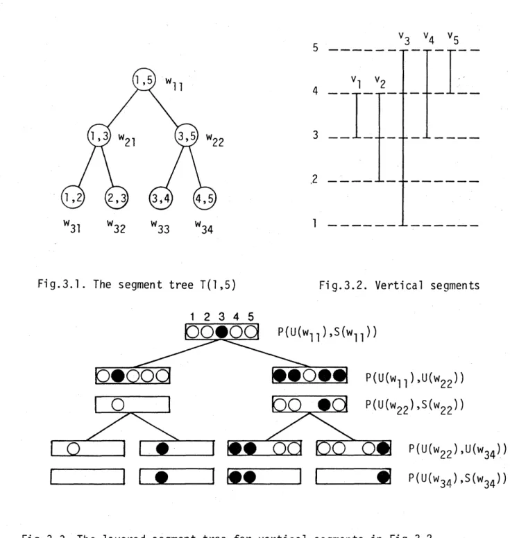
recall the segment tree due to Bentley [11. _For

_an

_integer _interval $(a,b$],

a

segment tree $T(a,b)$ _{consists of}

a

_root $w$ associated with interval $I(w)=(a,b$], and

in the

t-node of $\nu$, and $\emptyset\neq L(\nu)\cap I(w)\subset I(w)$.

A node $w$ is called

an

s-nodeof $\nu$ if

(i) $w$ is the root of $T(1,N)$ and $L(\nu)=I(w)$,

or

(ii) _the _parent _of $w$ is

a

t-node of $\nu$, and $I(w)\subseteq L(\nu)$

.

For each node $w$ of $T(1,N)$, let $S(w)$ be the set of $\nu\in V$ such that $w$ is

an

s-node of

$v$, and $U(w)$ be the set of $\nu\in V$ such that $w$ is

an

s-or

t-node of $\nu$

.

Note that

$S(w)\subseteq U(w)$. We keep the set $S(w)$ _by

a

_doubly _{linked list} _in _{increasing order.}

In the layered segment tree,

we

manipulate two kinds of ordered partitions. For each node $w$ of $T(1,N)$,

we

record

an

ordered partition $P(U(w),S(w))$. Also, for

each non-root node $w$,

we

record

an

ordered partition $P(U(w_{\pi}), U(w))$ where $w_{\pi}$ is

the parent of $w$ (note that $U(w)\subseteq U(w_{\pi})$) (Fig.3.3). Initially,

we

construct these

(8)

254

$v_{3}$ $v_{4}$ $v_{5}$

$21435$

$——————-v_{1,I_{-\underline{\ovalbox{\tt\small REJECT}}-\ovalbox{\tt\small REJECT}_{--}^{-\underline{\ovalbox{\tt\small REJECT}}_{----}^{-}}}^{-}}v_{2_{-}-}---I_{--}^{--}--$

$w_{31}$ $w_{32}$ $w_{33}$ $w_{34}$

Fig.3.1. The segment tree $T(1,5)$ _Fi_g.3.2. _{Vertical segments}

$P(U(w_{34}),S(w_{34}))$

Fig. 3.3. The layered segment tree for vertical segments in Fig.3.2

structures, which

can

be done in $0(n\log n)$ time _and space.

Let $h$ be

a

horizontal segment, whose interval with respect to abscissa is _{$[h_{/},h_{r}]$}

and whose ordinate is $h_{o}(1</l_{0}\leq N)$. Then the query for $h$

can

be executed

as

fol-lows. QUERY:

(i)

_find

$\nu\in V$ such that $\nu=\min\{\nu’|_{\nu’\in}V\cup\{n+1\}, h_{/}\leq\nu’\}$ by binary search;

if $\nu=n+1$_, then stop; otherwise, let $w$ be the root of $T(1,N)$;

(ii) $s_{i}:=find(\nu)$ with respect to the ordered partition $p(U(w),S(w))$;

report all the vertical segments $s\in S(w)$ such that $s_{i}\leq s\leq h_{r}$ by traversing the list representing $S(w)$;

(9)

-8-$f55$

(iii) _if $w$ is

a

leaf, then stop; otherwise, let $w_{\sigma}$ be

a

son

of $w$ with $h_{0}\in I(w_{\sigma})$;

$\nu:=find(v)$ with respect to the ordered partition $P(U(w), U(w_{\sigma}))$; return to (ii);

In the algorithm QUERY, each

_find

can

be executed in

a

constant time, hence Vaishnavi and Wood’s theorem [23] _is _obtained.

Theorem

3.1.

[23] _The _static _{orthogonal segment} _{intersection search} _problem

_can

be solved in $0(\log n+k)$ query time _and $O(n\log n)$ space where $k$

is

the number of

reported

intersections.

$\square$

3.2.

The insertion problem

In this problem, the set of vertical segments is updated by

_insertions.

Concerning queries, the algorithm QUERY given abOve works if

we

maintain respective ordered partitions correctly. We

now

give

an

algorithm INSERT which

inserts

a

vertical

seg-ment $\nu$ into the set with handling those ordered partitions correctly.

INSERT:

(i)

_find

$\nu^{*}\in V$such that $\nu^{*}=\min\{\nu’|_{\nu’\in}V\cup\{n+1\}, \nu\leq\nu’\}$ by binary search;

let $w$ be the root of $T(1,N)$;

(ii) _with respect to the ordered partition $P(U(w),S(w))$ ,

add$(\nu,\nu^{*})$; if _$w$ is

an

s-node of $\nu$, then split$(\nu)$;

if $w$ is

a

leaf, then return; otherwise, let $w_{\lambda}$ and $w_{\rho}$ be the

sons

of $w$;

with respect to the ordered partition $P(U(w), U(w_{\lambda}))$, $\nu_{\lambda}:=find(\nu^{*})$; add$(\nu,\nu^{*})$; if

$w_{\lambda}$ is

an s-or

t-node of $\nu$, then split$(\nu)$;

with respect to the ordered partition $P(U(w), U(w_{\rho}))$,

$\nu_{\rho}:=find(\nu^{*});add(\nu,\nu^{*})$; if $w_{\rho}$ is

an s-or

t-node of $\nu$, then split$(\nu)$;

(iii) _if $w$ is

a

t-node of $\nu$, then

if$L(\nu)\cap I(w_{\lambda})\neq\emptyset$ then $\nu^{*}:=\nu_{\lambda};w:=w_{\lambda}$ and return to (ii); if $L(\nu)\cap I(w_{\rho})\neq\otimes$ then $\nu^{*}:=\nu_{\rho};w:=w_{\rho}$ and return to (ii);

It is

seen

that, in the step (ii) _ofINSERT, $\nu^{*}$ for $\nu$

satisfies

the condition required

for executing add. It is then easy to show that the algorithm INSBRT correctly main-tains all the ordered partitions. We

now

consider the complexity of the above

algo-rithm.

Theorem

3.2.

An intermixed sequence of$0(n)$ _{queries and} _insertions

can

_be

exe-cuted in $O(n\log n+K)$ _time _and $O(n\log n)$ space, where $K$ is the total number of reported intersections.

Proof: The above algorithm obviously takes $O(n\log n)$ space,

so

that

we

consider

the time complexity. Suppose that, in the sequence, there

are

$q$ queries and $r$

inser-tions, where $q+r=O(n)$_. _In _the query step, $q$ queries except those parts for

find

operations

can

be executed in $0(q\log n+K)$ _{time. In the} _insertion _step, $r$ insertions

except those parts forfind, splitand add operations

can

be executed in $O(r\log n)$ time.

In all the steps, suppose that, for the ordered partition $P(U(w),S(w))$ of each node $w$ of $T(1,N)$, the

find

and splitoperations

are

executed $m_{0}(w)$ times,

an

the add operation is executed $l_{0}(w)$ times. Also, suppose that, for the ordered partition

$P(U(w_{\pi}), U(w))$ of each non-root node $w$ of $T(1,N)$, where $w_{\pi}$ is the parent of $w$,

(10)

256

the

_find

and split operations

are

executed $m_{1}(w)$ times, and the add operation is

exe-cuted $l_{1}(w)$ times. We consider that, for the root _$w,$ $m_{1}(w)=l_{1}(w)=0$. Then,

we

have $\sum_{w}(m_{0}(w)+m_{1}(w))=O((q+r)\log n)$ and $\sum_{w}(l_{0}(w)+l_{1}(w))=O(r\log n)$_,

where the summations

are

taken

over

all the nodes $w$ of $T(1,N)$.

Let

us

consider the complexity to execute sequences of $m,(w)$

find

and split

opera-tions and $l_{i}(w)$ add operations ($i=0,1$; all nodes $w$ of $T(1,N)$). Owing to the struc-ture of the segment tree, given $v\in V$ in

some

sequence,

we can

devise

a

procedure to

find

micro$(\nu)$ and number$(\nu)$ in the sequence in

a

constant time. We then

see

that,

from Theorem 2.4, these sequences

can

be executed in $0(n+ \sum_{w}\sum_{i}(m_{i}(w)+l_{i}(w)))$

time.

Thus, the whole sequence

can

be executed with the time complexity

$0((q \log n+K)+(r\log n)+n+\sum_{w}\sum_{i}(m_{i}(w)+l_{i}(w)))$_,

which is $0(n\log n+K)$

_.

$\square$

We next introduce

a

new

operation, called right. For

a

set $V$ of vertical segments, the operation right$(i,j)$

finds

$\nu\in V$ such that $\nu=\min\{\nu’|\nu’=n+1$

or

$[\nu’\in V,$ $i\leq\nu’$,

$j\in L(\nu’)]\}$

.

That is, right$(i,j)$

finds

the

first

segment in $V$that meets

a

line stretching

from

a

point $(i,j)$ in increasing abscissa. We

can

execute this right operation by

an

algorithm similar to that for the query. In this case,

we

do not need traversing the list of$S(w)$_,

so

_that _the _following _theorem _{is obtained.}

Theorem

3.3.

An intermixed sequence of$O(n)$ _right_{operations and} insertions

can

be executed in $O(n\log n)$ time _and $O(n\log n)$ space. $\square$

3.3.

The deletion problem

Using the operations link and find,

we can

efficiently solve the deletion problem. Given

a

vertical segment $\nu$ to be deleted,

we

do not

remove

all the elements

corresponding to $\nu$ from the data structure, but modify them

so

that $\nu$ will

no more

be reported in queries. Specifically,

on

each s-node $w$ of $\nu$,

we remove

$\nu$ out of

$S(w)$

.

_This _{makes the ordered} _partition _{$P(U(w),S(w))$} _update. _To _{obtain the}

updated ordered partition,

we

have only to execute link$(\nu)$. Combining this procedure with the algorithm QUERY,

we can

solve the deletion problem correctly. For

com-pleteness,

we

describe below

a

procedure for deleting

a

vertical segment $\nu$.

DELETE:

(i) _let $w$ be the root of $T(1,N)$;

(ii) _if $w$ is

an

s-node of $\nu$, then link$(\nu)$

with respect to the ordered partition $P(U(w),S(w))$;

(iii) _if $w$ is

a

t-node of $\nu$, then

let $w_{\lambda}$ and $w_{\rho}$ be the

sons

of $w$;

if $L(\nu)\cap I(w_{\lambda})\neq\otimes$ then _{$w:=w_{\lambda}$} and return to (ii);

if $L(\nu)\cap I(w_{\rho})\neq\otimes$ then _{$w:=w_{\rho}$} and return to (ii);

The following theorem

on

the complexity

_can

be obtained in

a

way similar to Theorem

3.2

(we

_use

_Theorem

_2.1

_in place of Theorem 2.4),

_so

that

we

omit the

proof.

(11)

10-$|^{v}$

S7

Theorem

3.4.

An intermixed sequence of $O(n)$ _{queries and} _deletions

can

_be

exe-cuted in $O(n\log n+K)$ _time and $O(n\log n)$ space, where $K$ is the total number of reported intersections. $\square$

4. Applications

(1) Finding the connected and biconnected components

of

an

intersection graph

_of

$n$

orthog-onalsegments [9].

An intersection graph ofsegment@ in the plane is obtained by representing each seg-ment by

a

vertex and connecting two vertices by

an

edge

iff

their corresponding seg-ments intersect. In [9], _{it is} _shown that, if

a

sequence of $O(n)$ _deletions _and _right

operations

can

be executed in $T_{D}(n)$ time and $S_{D}(n)$ space, the connected and

bicon-nected components of the intersection graph

can

be found in $0(T_{D}(n))$ time and $O(S_{D}(n))$ space. Hence, from Theorem 3.3,

we see

that the connected and

bicon-nected components

can

be found in $0(n\log n)$ time and $0(n\log n)$ space. Note _that,

only for finding the connected components, $0(n\log n)$-time and $O(n)$-space _optimal

algorithms, that

use

the plane-sweep technique,

are

known [41, [81.

Fig.4.1. Rectilinear regi

on

and

a

shortest Fig.4.2. Manhattan wiring

path between two points $S$ and $T$

in respect to $L_{1}$ metri

c

(2) _Finding

_a

_shortest _{path, in} _respect _to $L_{1}$ metric, between two $gi\nu en$ points in

a

rectil-inear region with $n$ edges [12] (see Fig.4.1).

A rectilinear region is

a

polygonal region whose edges

are

orthogonal segments, and may contain “holes. In [12], Kojima, Sato and Ohtsuki showed that the problem

can

be solved in $0(n\log n+T_{D}(n))$ time _and $0(S_{D}(n))$ space. Hence, it is

seen

from

Theorem

3.3

that the problem (2)

_can

_be _solved _in $O(n\log n)$ time and $O(n\log n)$

space.

(3) _{Discerning the existence}

_of

_a

_Manllattan wiring

_of

$n$ nets

on

a

single layer (Fig.4.2).

For $n$ pairs of points, called nets,

on a

grid,

a

wiring connecting all the pairs of

points by wires along grid lines is called

a

Manhattan wiring if the wires do not inter-sect

one

another and

no

wire has

more

than

one

bend. This problem

was

first

con-sidered by Raghavan, Cohoon and Sahni [201, who gave $0(n^{3})$-time algorithm. Masuda, Kimura, Kashiwabara and Fujisawa [171 _gave

_an

$0(n^{2})$-time algorithm by considering

an

intersection graph of possible wires and employing depth-first search

technique

on

that graph. Imai and Asano [91 _gave

_an

_efficient

_{implementation} _of_their

algorithm. Using the implementation with the data structure considered in this paper,

we

obtain

an

$O(n\log n)$-time algorithm for this problem (3).

be found quickly. Combining the techniques developed in [91 _{with the data structure} _for _the _deletion problem,

we can

show that this problem

can

be solved in $O(n^{3/2}\log n)$ time and $O(n\log n)$ space.

(5) Partitioning

a

$gi\nu en$ rectilinear region with $n$ edges into

a

minimum number

of

disjoint

rectangles (Fig.4.4).

Algorithms for this problem w\‘ere given in [151 _and [191. _The _main _step _of _those

algorithms is the problem (4), and

so we can

solve this problem in $O(n^{3/2}\log n)$ time and $0(n\log n)$ space.

The above problems

_are

applications of the algorithm for the deletion problem. Here, it should be noted that, concerning the problems $(1\sim 5)$_,

a

simpler data

struc-ture which gives the

same

results

as

above is given in Imai and Asano [91 by using proper structures of those problems. Also, note that

a

data structure similar to that in

[91 _is _{independently developed} _in _Lipski [141.

We below present two applications ofthe algorithm for the insertion problem.

(6) _{Finding the} _closure

_of

_a

_set

_of

$n$ rectangles with orthogonalsides [161.

A region $R$ in the $(x,y)$-plane is called closed if, for any pair of points $(x_{1},y_{1})$, $(x_{2},y_{2})\in R$ with $(x_{1}-x_{2})(y_{1}-y_{2})<0$ which

are

connected in $R$,

we

have $(x_{1},y_{2})$, $(x_{2},y_{1})\in R$. The unique smallest closed region containing $R$ is called the closureof$R$. In [161, Lipski and Papadimitriou considered the problem of finding the closure of

a

set of $n$ given rectangles with orthogonal sides (Fig.4.5).

The algorithm given in [161

_can

_be _implemented

_{so as}

_to

_run

_in $O(n\log n)$ time

and $O(n\log n)$ space _by _{using the} _algorithm _for _the insertion _{problem. Here,} _it

should be noted that, concerning the problem itself of finding the closure of

rectan-gles,

an

$O(n\log n)$-time _and $0(n)$-space _{optimal algorithm,} _which _is

_different

_from

that in [161 _and

_uses

_the _{plane-sweep technique,} _is _known [211.

(13)

-S5$

Fig.4.5. The cl

osure

of

a

set of rectangles

(7) Partitioning

a

rectilinear region into disjoint rectangles by adding $O(n)$ _chords

one

_by

one

in

a

$gi\nu en$ order.

This problem

can

be solved in $0(n\log n)$ time _and $0(n\log n)$ space. This

prob-lem

can

be used in several other problems. Here,

we

take up the problem of parti-tioning

a

rectilinear region into disjoint rectangles in such

a

way that the

sum

of the perimeters of those rectangles is

as

small

as

possible. This problem is known to be

NP-complete [111, and several heuristics have been considered. For example,

con-sider the following simple heuristic (see _Fig.4.6).

(a) (b)

Fig.4.6. Minimum perimeter partition into disjoint rectangl

es

(a) Concave points $P$ with di rected segments

$l_{P}$

(b) Approximate soluti

on

(i) _For _each

_concave

_point $P$ in the given rectilinear region, stretch

horizontal

and

vertical directed segments starting from $P$ into the region until they meet

an

edge of the region; take the shorter ofthe two, and denote it by $l_{P}$

.

(ii) Arrange all the

concave

points $P$ in the increasing order ofthe lengths of $l_{P}$

.

(iii) _{In that} order, stretch and add

a

segment starting from $P$ in the direction of $l_{P}$

(14)

-13-t60

until it meets

an

edge of the region

or

another segment that has

aiready

been added to the region.

In this heuristic algorithm, the main step isjust the problem (7), and

so

this heuristic

can

be executed in $O(n\log n)$ time _and $O(n\log n)$ space.

Acknowledgment

The authors thank Professor Y. Kambayashi of Kyoto University for informing them ofthe paper [211.

References

[11 _J. _L. _Bentley: _Solutions _to _Klee’s _{Rectangle Problems, unpublished note,}

Depart-ment ofComputer Science, Carnegie-Mellon University,

1977.

[21 _B. _Chazelle: _Filtering _Search: _A _New _Approach _to _{Query-Answering.} Proceedings

of

the 24th Annual IEEE Symposium

on

Foundations

_of

Computer Science, Tucson, 1983, pp.122-132.

[31 _H. _{Edelsbrunner:} Dynamic Data Structures for Orthogonal Intersection Queries.

Report 59, Institut f\"ur Informationsverarbeitung, Technische Universitat Graz,

1980.

[41 _H. _{Edelsbrunner,} _J.

_van

_Leeuwen, _{T. Ottmann} _{and D.} _Wood: _Connected

Com-ponents of 0rthogonal

Geometric

Objects. Report 72, Institut f\"ur Informa-tionsverarbeitung, Technische Universitat Graz,

1981.

[5] _H. _N. _{Gabow and} _R. _{B. Tarjan: A} _Linear-Time _Algorithm _for

_a

Special Case of

Disjoint Set Union, July 1982, submitted to Journal

_of

Computer andSystem

Sci-ences

(also _cf. _{Proceedings of the} _15th _Annual _ACM _Symposium

_on

_Theory _of

Computing, Boston, 1983, pp.246-251).

[6] _J. _E. _Hopcroft _and

_J.

_{D. Ullman: Set} _{Merging Algorithms.} _{SIAM Journal}

_on

Computing, Vol.2 (1973), pp.294-303.

[7] _H. _Imai _{and T.} _Asano: _An

_Efficient

_Algorithm _for _Finding

_a

_Maximum _Matching

of

an

Intersection Graph of Horizontal and Vertical Line Segments. Papers

_of

the Technical Group

on

Circuits

andSystems, CAS 83-143, Institute of Electronics and Communication Engineers ofJapan,

1983.

[81 _H. _Imai _and _{T. Asano:} _Finding _{the Connected} _Components _and

_a

_Maximum

Clique of

an

Intersection Graph of Rectangles in the Plane. Journal

_of

Algo-rithms, Vol.4 (1983), pp.310-323.

[91 _H. _Imai _and _T. _Asano:

_Efficient

_Algorithms _{for Geometric} _Graph _Search

Prob-lems. Research Memorandum RMI $83- 05$_, Department of Mathematical

Engineer-ing and

Instrumentation

Physics, University ofTokyo,

1983.

[101 _H. _Imai _and _T. _Asano: _{Dynamic Orthogonal} _Segment _{Intersection Search.}

Research Memorandum RMI $84- 02$_, Department of Mathematical Engineering

and Instrumentation Physics, University ofTokyo,

1984.

[111 _D. _{S. Johnson: The} _{NP-Completeness} _Column: _{An Ongoing} _Guide. _Journal

_of

Algorithms, Vo1.3 (1982), pp.

182-195.

[121 _{I. Kojima,} _M. _Sato _and _{T. Ohtsuki:} _A _Shortest _Path _Algorithm

_on

_a

_Planar

Rec-tilinear Region (in _{Japanese). Papers}

_of

_the $Tec/mical$ Group

on

Circuits _and

(15)

-14-$d\mathcal{L}$

Sl

Systems, CAS 83-205, Institute of Electronics and Communication Engineers of Japan,

_1984.

[13]

_W.

_Lipski, _Jr.: _Finding

_{a Manhattan}

_Path _and _{Related Problems.} _Networks,

Vo1.13 (1983), pp.399-409.

[14] _W. Lipski, Jr.: An $O(n\log n)$ Manhattan Path Algorithm. Research Report 141,

Laboratoire de Recherche

en

Informatique, Universite de Paris-Sud,

1983.

[15] _W. Lipski, Jr., E. Lodr, F. Luccio, C. Mugnai and L. Pagli: On Two Dimensional Data 0rganization II. Fundamenta Informaticae, Vo1.2 (1979),

pp.245-260.

[161 _W. Lipski, Jr., and C. H. Papadimitriou: A Fast Algorithm for Testing for Safety and Detecting Deadlocks in Locked Transaction Systems. Journal

_of

Algorithms, Vo1.2 (1981), pp.211-226.

[17] _S. Masuda, S. Kimura, T. Kashiwabara and T. Fujisawa: On Manhattan Wiring Problem (in Japanese). Papers

_of

the Technical Group

on

Circuits and Systems, CAS 83-20, Institute of Electronics and Communication Engineers of Japan,

1983.

[181 _{B. M.} McCreight: Priority Search Trees. Technical Report CSL-81-5, Xerox Palo Alto Research Centers,

1982.

[19] _T. Ohtsuki, M. Sato, M. Tachibana and S. Torii: Minimum Partitioning of Recti-linear Regions (in Japanese). Transactions

_of

_Information

Processing Society

_of

Japan, Vol.24, No.5 (1983), pp.647-653.

[201 _R. _Raghavan, _{J. Cohoon} _and _{S. Sahni: Manhattan} _and _Rectilinear _Wiring.

Techn-ical Report 81-5, Computer

Science

Department, University ofMinnesota,

1981.

[211 _B. $Soisalon- So|ninen$ and D. Wood: An Optimal Algorithm forTesting for Safety

and Detecting Deadlocks in Locked Transaction Systems. Proceedings

_of

the

1st

$ACM$

Conference

on

Principle

of

DatabaseSystem, 1982, pp.

108-116.

[221 R. E. Tarjan: Data Structures and Network Algorithms. Society for Industrial and