A New Method of Model Selection for Value Function
Approximation in Reinforcement Learning
Takayuki Akiyama
∗, Hirotaka Hachiya, and Masashi Sugiyama
Department of Computer Science, Tokyo Institute of Technology
Abstract: In reinforcement learning, the use of a linear model for value function approximation is promising due to its high scalability to large-scale problems. When we use such a method in practical reinforcement learning problems, how we choose an appropriate model for good approxi-mation is quite important because the approxiapproxi-mation performance heavily depends on the choice of the model. In this paper, we propose a new method of model selection with sample data, and we demonstrate the effectiveness of the proposed method in chain walk and inverted pendulum problems.
1
Introduction
Policy Iteration is a standard framework of rein-forcement learning to obtain the optimal policy by iteratively performing policy evaluation (calculating the state-action value function of the current policy) and policy improvement (updating the current policy with the value function)[1]. But generally it takes a lot of time to evaluate the current policy if the num-bers of states and actions are large, and it is hard to evaluate the current policy accurately if the state or action spaces are continuous. To overcome these difficulties, it is necessary to approximate policy eval-uation.
Least-Squares Temporal Difference Q learning (LS-TDQ), in which a linear model and the least-squares method are used for state-action value function ap-proximation, has been proposed for approximate pol-icy iteration [2]. LSTDQ has several nice features, e.g., it is simple and its implementation is easy. But actually the performance of LSTDQ heavily depends on the choice of the linear model and a systematic method of selecting an appropriate linear model has not been proposed so far. To cope with this problem, we propose a model selection method by using the Cross Validation method and apply this method for every approximate policy evaluation step. We demon-strate the usefulness of the proposed model selection method by chain walk and inverted pendulum prob-lems.
∗Department of Computer Science, Tokyo Institute
of Technology, 2-12-1, O-okayama, Meguro-ku, Tokyo, 152-8552, Japan E-mail:akiyama@sg.cs.titech.ac.jp, hachiya@sg.cs.titech.ac.jp, sugi@cs.titech.ac.jp
2
Reinforcement Learning
Problem
Reinforcement Learning [1] deals with the problem of learning to get as many rewards as possible from interaction between an agent and an environment de-fined as a Markov decision process (MDP). At first we formulate the reinforcement learning problem.
2.1
Markov Decision Process
We define a Markov decision process (MDP) which represents an environment and consists of five ele-ments (S, A, PT, R, γ). Here, S is a set of states, A
is a set of actions (we generally deal with continuous state and action spaces here), PT(s0|s, a) is the
proba-bility density function of making a transition to state
s0 when taking action a in state s, R(s, a, s0) is the reward function for the transition from s to s0 by tak-ing action a, and γ∈ (0, 1] is the discount factor. We also define the agent’s policy as π(a|s) which means the probability density of taking action a in state s. Let us define the R function as the expected reward function when taking action a in state s:
R(s, a)≡ E
PT
[R(s, a, s0)].
2.2
State-Action Value Function
The state-action value function (called the Q func-tion) has a role of evaluating a policy. The Q function
人工知能学会研究会資料 SIG-DMSM-A703-09 (2/29)
of policy π is defined as Qπ(s, a)≡ E at∼π st∼PT "∞ X t=1 γt−1rt|s1= s, a1= a #
for all s ∈ S and a ∈ A, the value of which is the expected discounted sum of rewards from the interac-tions after taking action a in state s. In the above definition, Eat∼π,st∼PT means the expectation over
{st, at} for 1 ≤ t ≤ ∞ under π(at|st) and PT(st|st, at).
2.3
Policy Iteration
Based on the Q function defined above, let us define the purpose of reinforcement learning formally. The goal is to obtain the optimal policy π∗ defined as
π∗≡ δ(a − argmax
a0
Q∗(s, a0)),
where δ(x) (x∈ R) is the Dirac delta function. Q∗(s, a) is the optimal Q function defined as
Q∗(s, a)≡ max
π Q π(s, a).
To obtain this optimal policy, we use the policy itera-tion method in which after initializing the agent’s pol-icy arbitrarily we iterate polpol-icy evaluation and polpol-icy improvememt. Policy evaluation means to calculate the Q function of policy π, and policy improvement means softmax update of policy π defined as
π0(a|s) = exp(Q
π(s, a)/τ )
R
a0exp(Qπ(s, a0)/τ )da0
,
where the variable τ is called temperature by which we can control the randomness of the updated policy.
2.4
Value Function Approximation by
Using a Fixed Linear Model
In this subsection, we consider approximating the Q function of the current policy π with sample data. For approximating the Q function, we use the following linear model: b Qπ(s, a; θ)≡ B X b=1 θbφb(s, a) = θ>φ(s, a),
where φ(s, a) = (φ1(s, a), . . . , φB(s, a))>are the fixed
basis functions, > denotes the transpose, B is the number of basis functions, and θ = (θ1, . . . , θB)> are
model parameters. For N -step transitions, we ideally
want to learn the parameters θ so that the approxi-mation error G is minimized:
θ∗≡ arg min θ G, G≡ E PI,π,PT " 1 N N X n=1 g(sn, an; θ) # , g(s, a; θ)≡ ³ b Qπ(s, a; θ)− Qπ(s, a) ´2 ,
where g(s, a; θ) is a cost function corresponding to the approximation error of bQπfor each pair (s, a) and
EPI,π,PT denotes the expectation over{sn, an}
N n=1
fol-lowing the initial probability density PI(s1), policy
π(an|sn) and transition probability PT(sn+1|sn, an).
A fundamental problem of the above formulation is that the target function Qπ(s, a) can not be observed
directly. To cope with this problem, we use the Bell-man residual cost function [2] defined by
gBR(s, a; θ) ≡³Qbπ(s, a; θ)− R(s, a) − γ E π(a0|s0) PT(s0|s,a) h b Qπ(s0, a0; θ) i ´2 .
Next we consider learning the parameters θ with sam-ple data so that the approximation error G is mini-mized. We suppose that a data set consisting of M episodes of N steps is available. The agent initially starts from a randomly selected state s1following the
initial probability density PI(s) and chooses an
ac-tion based on policy π(an|sn). Then the agent makes
a transition following PT(sn+1|sn, an) and receives a
reward rn(= R(sn, an, sn+1)). This is repeated for N
steps—thus the training dataD is expressed as
D ≡ {dm}Mm=1,
where each episodic sample dm consists of a set of
4-tuple elements as
dm≡ {(sm,n, am,n, rm,n, sm,n+1)}Nn=1.
With this sample data, we can obtain a consistent estimator bθ (i.e., the estimated parameters converge
to the optimal values as the number of episodes M goes to infinity): bθ ≡ arg min θ b G, b G≡ 1 M N M X m=1 N X n=1 bgm,n, bgm,n≡ bgBR(sm,n, am,n, rm,n; θ,D),
bgBR(s, a, r; θ,D) ≡³Qbπ(s, a; θ)−r− γ |D(s,a)| X s0∈D(s,a) E π(a0|s0) [ bQπ(s0, a0; θ)] ´2 ,
where D(s,a) (⊂ D) is a set of 4-tuple elements
con-taining state s and action a.
A practical problem of this approach is that the per-formance of the above method depends on the choice of the basis functions. In the next section, we propose a new method of selecting an appropriate set of basis functions.
3
A New Model Selection
Method by Using CV
The main idea of our model selection method is to select a model which minimizes the approximation er-ror G from some model candidates. For that purpose we estimate G by using Cross Validation (CV). A ba-sic idea of CV is to divide the training dataD into a ‘training part’ and a ‘validation part’. Then the pa-rameters θ is learned from the training part and the approximation error is estimated using the validation part. The detailed procedure of the model selection method is described below.
(The procedure of model selection) 1. Prepare a set of model candidates M.
M = {M1,M2, . . . ,MC}.
2. Estimate the approximation error G with the K-fold Cross Validation method. We divide sample dataD into K disjoint subsets {Dk}Kk=1of
(ap-proximately) the same size. For simplicity, we assume that M/K is an integer. Let bθk be the parameters learned from {Dk0}k06=k for model
MX (X = 1, 2, . . . , C). Then the
approxima-tion error G is estimated by
b GKCV= 1 K K X k=1 b GkKCV, where b GkKCV= K M N ×X dm∈Dk N X n=1 bgBR(sm,n,am,n,rm,n;bθ k ,Dk).
We estimate the approximation error for all mo-del candidates by the above K-fold CV method.
3. Select the model cM with the minimum esti-mated approximation error.
c M = argmin M b GKCV.
4
Experimental Results
In this section, we demonstrate the usefulness of our model selection method by simple chain walk and inverted pendulum problems.
4.1
Chain Walk
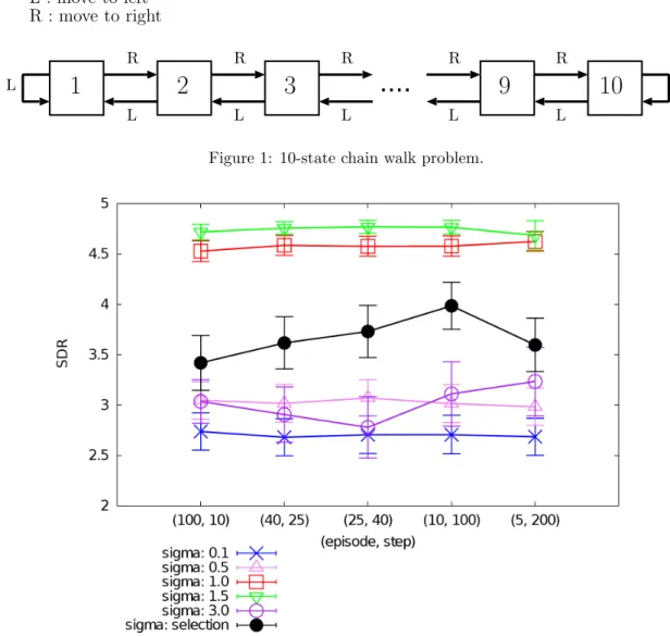
As shown in Figure 1, an agent is on one of the states from 1 to 10 and at each state the agent can select two actions: moving to left or right (we define the two actions a(1), a(2) as ‘R’, ‘L’). But the
proba-bility of moving to the direction to which the agent intends to move is set at 0.9. For example, if the agent takes action ‘R’ at state 2, the next state is 3 with probability 0.9, and 1 with probability 0.1. The agent can get reward +0.5 if it reaches state 3 or 8, 0 reward otherwise. The discounted factor is set at 0.95. In this experiment, we use 10 Gaussian functions as the basis functions for Q function approximation.
φσ2(i−1)+j(s, a) = I(a = a(j))exp µ −(s− ci)2 2σ2 ¶ for 1≤ i ≤ 5, 1 ≤ j ≤ 2, where I(x) = ( 1 (if x = 0), 0 (if x6= 0), {c1, c2, c3, c4, c5} = {2, 3, 6, 8, 9}.
Here the Gaussian width σ is the model. We prepare 5 different models:
σ∈ {0.1, 0.5, 1.0, 1.5, 3.0}.
In each iteration, we gather 1000 samples. We tested different sampling patterns by changing the number of episodic samples and the number of steps in each episodic sample.
(episode, step) = (100, 10), (40, 25), (25, 40), (10, 100), (5, 200).
....
L R R R R R R L L L L LL : move to left
R : move to right
1
2
3
9
10
Figure 1: 10-state chain walk problem.
Figure 2: Sum of discounted rewards for each model (chain walk).
We use 5-fold CV for model selection. In the policy update, we use softmax update defined as
π0(a|s) = exp( bQ
π(s, a)· T )
P2
j=1exp( bQπ(s, aj)· T )
,
where T denotes the current iteration number (T ≥ 1). After we obtained the learned policy by iterating policy evaluation and improvement for 5 times, we observe the sum of discounted rewards (SDR) from interactions with the environment for 100 steps with the learned policy for all 10 initial states. By repeat-ing this experiment for 60 times, 60× 10 SDRs are observed and we calculate average and the standard deviation.
The results are shown in Figure 2 (the value of the standard deviation is divided by 4 for clear
visibil-ity). The graph shows that we can obtain good per-formances by applying our model selection method.
4.2
Inverted Pendulum
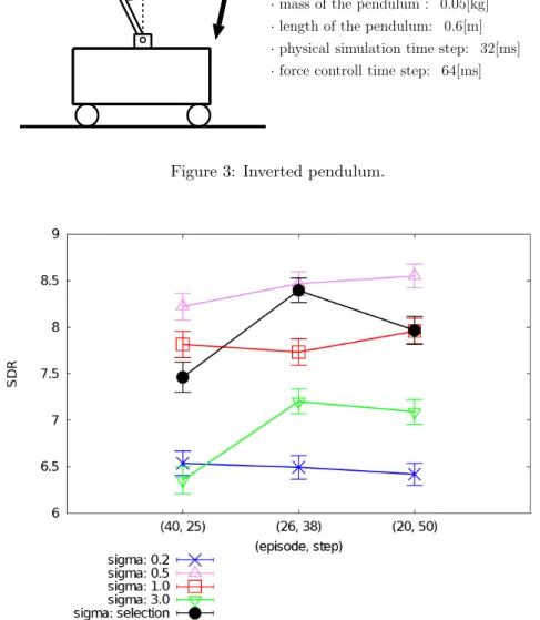
The inverted pendulum problem is a standard re-inforcement learning test bet [1, 3]. The goal of this problem is to keep balancing a pendulum by moving a cart to which it is attached (Figure 3). The state of the pendulum consists of the angle θ and the angu-lar velocity ˙θ computed as 10(θ− θ0), where θ means the current angle and θ0means the previous angle (64 msec before):
θ
(Parameter Settings) · mass of the cart : 1.0[kg] · mass of the pendulum : 0.05[kg] · length of the pendulum: 0.6[m] · physical simulation time step: 32[ms] · force controll time step: 64[ms]
Pendulum
Cart
Figure 3: Inverted pendulum.
Figure 4: Sum of discounted rewards for each model (inverted pendulum).
At the beginning of each time step, the agent is al-lowed to take 3 actions : left force (−20[N]), no force (0[N ]), right force (+20[N ]) (we define the three ac-tions a(1), a(2), a(3)as -20, 0, 20). The reward function
is defined as
1 2cos
2
(θ).
In this experiment, we used Webots1 as a physical
simulation software.
As the basis functions for Q function approximation,
1http://www.cyberbotics.com/
we use 30 basis functions defined as follows.
φσ3(i−1)+j(s, a) = ( I(a = a(j)) (if i = 1) I(a = a(j))exp³−ks−cik2 2σ2 ´ (if i6= 1) for 1≤ i ≤ 10 , 1 ≤ j ≤ 3, where {c2, . . . , c10}={(− π 4,−1), (− π 4, 0), (− π 4, 1), (0,−1), (0, 0), (0, 1), (π 4,−1), ( π 4, 0), ( π 4, 1)}, The model candidates are
In data sampling, we tested 3 sampling patterns: (episode, step) = (40, 25), (26, 38), (20, 50).
The initial state of each episode is always set at the state
(θ, ˙θ) = (0, 0).
We use 2-fold CV for model selection. The softmax policy update rule and the value of γ are the same as the chain walk experiment. After we obtained the learned policy by 3 iterations, we observe 10 SDRs from 100 step interactions with the environment from the initial state (0, 0). This experiment is executed for 30 times, and we take the average and the standard deviation of the observed 30× 10 SDR values.
The result is shown in Figure 4 (the value of the standard deviation is divided by 10 for clear visibil-ity). The graph shows that similar to the chain walk experiment, we can obtain nice performances.
5
Conclusions
How we approximate state-action value function ac-curately is one of the most important topics in rein-forcement learning since this directly influences the performance of the policy iteration method. A diffi-culty of approximating the Q function by using a lin-ear model is that the model has to be selected appro-priately for good approximation, but generally the ap-propriate model depends on each reinforcement learn-ing problem. In this paper, we proposed a new model selection method and have shown the usefulness of our model selection method by two experiments.
Reference
[1] Richard S. Sutton, Andrew G. Barto: ”Re-inforcement Learning: An Introduction”, MIT Press, Cambridge, MA, (1998)
[2] Michail G. Lagoudakis, Ronald Parr: ”Least-Squares Policy Iteration”, Journal of Machine Learning Research, 4, pp.1107–1149, 2003 [3] Esogbue, A.O., Hearnes, W.E. and Song, Q:
”A Reinforcement Learning Fuzzy Controller for Set-Point Regulator Problems”, Proceedings of the IEEE 5th International Fuzzy Systems Con-ference, New Orleans, LA, September 8-11, 1996, pp. 2136–2142.