Top-down Zooming Diagnosis of Logic Programs

147

Top-down

_Zooming

_{Diagnosis ofLogic Programs}

Machi

MAEJI

Tadashi

_KANAMORI

前地 真知 _{金森 直}

Central Research Laboratory

Mitsubishi

Electric

Corporation

8-1-1,

Tsukaguchi-IIonmachi

Amagasaki, Hyogo,

Japan 661

Abstract

This paper presents a

new

diagnosis _{algorithm for}

_Prolog

_{proglams. Bugs are}

located

by _{tracing either proof trees}

_or

_{search trees in a}

top-down mallIler.

Human programmers

just need to

answer

“Yes”

or

“No” forqueries _{issued durin theto -d} queries_{about atoms with the}

_same

_pIedicates

_are

issued contirrually so thatnot onl

$g$ $e$ op-

own tracing. Moreover,

containing

bugs ar

identified

more

_{quickly but also queries}

_are

_{easier for hu}no on$y$segments

to

_answer.

_{An outline ofan implementation of}

the diagnosis algorithm is shown as $we\mathbb{I}$. or

uman

programmers

Keywords :

_{Program Diagnosis,}

_Debugging,

_{Prolog, Program}

Analysis.

Contents

1.

_Introduction

2.

Diagnosis

ofLogic

Programs

2.1 Bugs of

Prolog Programs

2.2 “trace” and “spy”

_Commands

_in

_{DEC-10 Prolog}

2.3 Proof Tree and

Search

Tree

3. Top-down

_{Zooming Diagnosis}

_ofLogic

_Programs

3.1 Unexpected

_Success

_{and Unexpected Failure}

3.2 Top-down

_Diagnosis

_Algorithm

3.3 Top-down

_{Zooming Diagnosis}

_Algorithm

4. Implementation of_{the Top-down}

_{Zooming Diagnosis}

_Al

orithm

4.1

_{Consideration}

_on

_Space

_Efliciency

$g$

4.2

_{Consideration}

_{on Time Effciency}

4.3

_{Consideration}

_on

_Query 5.

_Discussion

6.

Conclusions

Acknowledgements

References

数理解析研究所講究録 第 655 巻 1988 年 147-166

1. Introduction

Though it is saidthat the programming language Prolog is a muchhigherlevellanguage

so that writing programs in Prolog is much easier than the conventional languages, still it

remains as an important task to debug Prolog programs. Several conventional debugging

tools, e.g., “trace“ and “spy” commands, areprovided in DEC-10 Prolog. Inaddition,several

more advanced debugging tools havebeenstudied bytaking advantages of thecharacteristics

oflogic programs, e.g., “algorithmic debugging“ by Shapiro [10], “declarative debugging” by Lloyd [6], and “rational debugging” by Pereira [8]. In these approaches, they all

assume

a

device, caUed “_{oracle”, which always}

answers

_{correctly forqueries issued during the}diagnosis. If the device is a human programmer, not only should the diagnoser be efficient in the query

number complexity but also should the queries be easy to answer for human

programmers.

Attention should be paid to both of these pointswhen anefficient debuggingtool for human

programmers is aimed at.

This paper presents a new diagnosis algorithm for Prolog programs. Bugs are located

by tracing either proof trees or search trees in a top-down

manner.

Human

programmers

just need to answer “Yes” or “No” for queries issued duringthe top-downtracing. Moreover,

queriesabout atoms with thesamepredicatesareissuedcontinuallysothat not onlysegments

containing bugs areidentifiedmorequickly but alsoqueries are easierfor human

programmers

to answer.

This paper is organized as follows: First in Section 2, we will present two kinds of

program’s bugs, and two DEC-10 Prolog commands, “trace” and “spy”. Next in Section 3,

we will show a top-down diagnosis algorithm in the “trace“

manner.

Then we will improve

the diagnosis algorithm into the one in the “spy” manner. Last in Section 4, we will show

an implementation with efficiency consideration.

The following sections assume familiarity with the basic terminologies offirst order

logic such as term, atom (atomic formula), clause (definite clause), substitution, most

gen-eral unifier (m.g.$u.$) and so on. Knowledge of the semantics of Prolog such as Herbrand

interpretations, least Herbrand models and transformation $T_{P}$

as

sociated with program $P$

is also assumed. The syntax ofDEC-10 Prolog is followed. Syntactical variables are $X,$ $Y$,

$Z$ for variables, $A,$ $B$ for atoms, $L,$ $G$ for atom sequences, and $\theta$ for substitution, possibly

with primes and subscripts. A program is a finite set of

_definite

$cla$

uses

of the form $A$ :-$B_{1},$ $B_{2},$

$\ldots,$$B_{k}$ $(k\geq 0)$, where $A,$ $B_{1},$ $B_{2},$ $\ldots,$ $B_{k}$ are atoms. The atom $A$ and the atom

sequence $B_{1},$ $B_{2},$

$\ldots,$ $B_{k}$ are caUed the headand the body of this clause, respectively. The

empty atom sequence is denoted by $\square$.

2. Diagnosis of Logic Programs

2.1 Bugs ofProlog Programs

Even ifa very higher level programming language like Prolog is used, we are likely to

write buggy programs.

Example 2.1.1 The following is a

program

of quick sort. It contains a wrong clause in the

14

$g$

qsort$([], [ ])$.

qsort($[X|L]$, LO) :-partition($L,$ $X$, Ll, L2), qsort(Ll, L3),

qsort(L2, L4), append(L3, [X$|L4]$, LO).

partition([X$|L],$ $Y$, Ll, $[X|L2]$) :- $Y\leq X$, partition(L, $Y$, Ll, L2).

partition($[X|L],$ $Y,$ $[X|L1]$, L2) :- $X\leq Y$, partition(L, $Y$, Ll, L2).

partition([], X, [], [ ]).

append($[X|L1]$,L2, $[X|L3]$) $:-append$($Ll$, L2, L3).

append$([], L, [ ])$. % append$([], L, L)$.

Example 2.1.2 The following is a programofpermutation. It misses arecursiveclause with the predicate “insert”, which is shown at the right of the symbol “%’’.

perm$([], [ ])$.

perm$([X|L], N):- perm(L, M),$ $insert(X, M, N)$.

insert(X, $L,$ $[X|L]$).

% insert(X, $[Y|M],$ $[Y|N]$) _{$:- insert(X, M, N)$}.

WhenaPrologprogram is buggy, we experience differences between the actual behavior when executed and the intended modelin our mind.

The algorithm for executing pure Prolog program is the usual ordered linear, that

always selects the leftmost atom from atom sequences to be resolved. When $G\theta$ is obtained

by executing an atom sequence $G$ in a program $P$, the instance $G\theta$ is caUed a computed

solution (or a solution, for simplicity) of$G$ in $P$. A program is called a terminatingprogram

when theexecution of any atom in theprogramterminates finitely. In this paper, theprogram

considered are restricted to terminating one.

Let $G$ be an atom sequence and $M$ be an intended Herbrand interpretation in our

mind. $G$is said to be validin $M$ ifall ground instances of$G$ are true in M. $G$is said to be

invalidin $M$ ifsome ground instance of$G$is false in $M$

.

What computed solutions should be returned when an atom sequence is executed in

a program that is correct w.r.$t$

.

an intendedinterpretation $M$? An atom sequence is called

an intended solution of$G$ with respect to $M$ when it is an instance of$G$ and valid in $M$. A

ground atom sequence is called a missed solution of$G$in $P$w.r.t. $M$, when it is an intended

solution of $G$ w.r.t. $M$ but not an instance of computed solution of $G$ in $P$. Then, we say

that the execution-result

_of

$G$ in $P$ is correctw.r.$t$

.

$M$ when

(a) computed solutions of$G$in $P$are all intended solutions w.r.$t$. $M$, and

(b) there is no missed solution of$G$ in $P$ w.r.t. $M$

.

Otherwise, we say that the execution-result

_of

$G$ in $P$ is incorrect w.r.$t$

.

$M$

.

When the

execution-results of all atom sequences in a program are correct w.r.$t$

.

$M$, we say that this

program is correct w.r.$t$. $M$

.

Otherwise we say that this program is“incorrectw.r.$t$

.

$M$.

When a program is incorrect w.r.$t$. an intended interpretation, what kinds ofbugs are

there in the program? We will define two kinds of bugs in incorrect

programs

following

Shapiro [10] and Lloyd [6].

Definition 2.1.1 –wrong clause instance –

Let $P$ be a program and $M$ be an intended interpretation. An instance A:-L’ of a

clause in $P$is called a wrong clause instance in $P$w.r.t. $M$ when

(a) $A$ is invalid in $M$, and

Example 2. 1. 3 In the program of Example 2.1.1, append$([], [1], [ ])$” _{is a}

wrong

_clause instance, because append$([], [1], [])$“ _{is invalid w.r.}$t$. our intention.

Definition 2.1.2 –uncovered atom –

Let $P$ be a program and $M$ be an intended interpretation. An atom $A$ is caUed an

uncovered atomin $P$w.r.t. $M$, when there exists some ground instance $A\theta$ such that

(a) $A\theta$is true in $M$, and

(b) for any ground instance $A\theta:- L$’ ofa definite clause in $P$, the body $L$ is false in $M$.

Example

_2.1.4

In the program of Example 2.1.2, insert$(2, [1], X)$ _is an uncovered atom,

because insert$(2, [1], [1,2])$ is true in $M$, and thereis no clausein the program whosehead

is unifiable with the atom.

Then, the following theorem

ensures

that we can attribute incorrectness of programs

to either a wrong clause instance or an uncovered atom (cf. Shapiro [10], Lloyd [6]). Theorem 2.1

Let $P$ be a terminatin_$g$ program and $M$ be an in$t$en$ded$ interpretation. $T\Lambda$en $P$ is

incorrect lv.t.$t$. $M$ ifan$d$ only ifeither tlrere is a wron_$g$clauseinstance in $P$ _lv.t.$t$. $M$ orther_$e$

is an un$co$vered a tom in $Pw.r.t$

.

$M$

.

Proof.

$\cdot$ First we wiu show the “if” part. Suppose that the

program

$P$is correct.

If there is a wrong clause instance A:-L’ in $P$ w.r.t. $M$, the atom $A$ is invalid in $M$

and the atom sequence $L$ is valid in $M$

.

Because theprogram $P$iscorrect, $L$ is an computed

solution of itself in $P$. By using the clause instance A:-L’, $A$ is an computed solution of

itselfin $P$, so that $A$ is valid in $M$ due to the correctness of$P$

.

Thisfact contradicts the fact

that $A$ is invalid in $M$

.

If there is an uncovered atom $A$ for $P$ w.r.t. $M$, there is a ground instance $A\theta$ such

that $A\theta$ is true in _$M$, and for any ground instance $A\theta:- L$“ ofa definite clause in $P,$ $L$ is

false in $M$. Then, such $L$ has no computed solution due to the correctness of $P$

.

Hence $A\theta$

has nocomputed solution, but $A\theta$is true in $M$, which means that $A\theta$is amissed solution of

$A$

.

This fact contradicts the fact that $P$ is correct.

Next, we will show the contrapositive of the “only if“ part. Suppose that there is

neither a wrongclauseinstance nor an uncovered atom. For everyground atom $A$in_{$T_{P}(M)$},

there is a ground instance A:-L’ ofsome clause in $P$ such that $L$ is valid in $M$

.

Because

A:-L“ _{is not} a wrong _{clause instance,} $A$ is valid in $M$, so that $A$ E $M$

.

Hence$T_{P}(M)\subseteq M$ holds. For every groundatom $A$in$M$, because $A$isnot anuncovered atom, thereis aground

instance A:-L’ ofsome clause in $P$such that $L$ is true in $M$, so that _{$A\in T_{P}(M)$}

.

Hence

$T_{P}(M)\supseteq M$ holds. Therefore$T_{P}(M)=M$, that is, $M$ is a fixpoint of$T_{P}$

.

(See [5] for the

transformation $T_{P}$ associated with

program

$P.$) Because $P$ is terminating, and the finite

failure set must be included in the complement of the greatest fixpoint [5], thereisjust

one

fixpoint of$T_{P}$, i.e., the least Herbrand model of $P$. Hence, $M$ is the least Herbrand model

of$P$, which obviously means that $P$is correct w.r.$t$

.

$M$

.

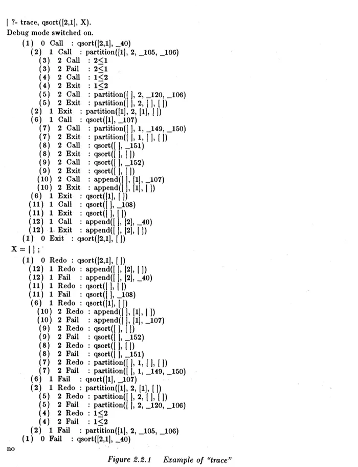
2.2 “trace” and “spy” Commands in DEC-10 Prolog

When we experience differencesbetween the program behaviorandits intended model,

we often trace and examine the execution using a “tracer“. Let us trace the execution ofan

atom qsort$([1,2], X)$ _in the

program

of Example 2.1.1

using

the “trace” command in

DEC-10 Prolog. The numbers preceded by the underline “

–

”

_are

_{the inner variables generated}

151

$|?-$trace, qsort$([2,1], X)$.

Debugmodeswitched on.

(1) $0$ Call : qsort$([2,1], -40)$ (2) 1 Call : partition([l], 2, $-105,$ $-106$) (3) 2 Call : $2\leq 1$ (3) 2 Fail : $2\leq 1$ (4) 2 Call : $1\leq 2$ (4) 2 Exit : $1\leq 2$ (5) 2 Call : partition$([], 2, -120, -106)$ (5) 2 Exit : partition([], 2, [], []) (2) 1 Exit : partition([l], 2, [1], [ ]) (6) 1 Call : qsort([l],$-107$) (7) 2 Call : partition($[]$, 1,

$–$

(7) 2 Exit : partition([], 1, [], [ ]) (S) 2 Call : qsort$([], -151)$ (8) 2 Exit : qsort$([]$, []$)$ (9) 2 Call : qsort$([], -152)$ (9) 2 Exit : qsort$([]$, [ ]$)$ (10) 2 Call : append$([], [1], -107)$ (10) 2 Exit : append$([], [1], [ ])$ (6) 1 Exit : qsort$([1|, [ ])$ (11) 1 Call : qsort$([], -108)$ (11) 1 Exit : qsort$([]$, [ ]$)$ (12) 1 Call : append$([], [2], -40)$ (12) 1 Exit : append$([], [2], [ ])$ (1) $0$ Exit : qsort$([2,1], [ ])$ $X=[]$ ; (1) $0$ Redo : qsort$([2,1], [ ])$ (12) 1 Redo : append$([], [2], [ ])$ (12) 1 Fail : append$([], [2], -40)$ (11) 1 Redo : qsort$([]$, [ ]$)$ (11) 1 Fail : qsort$([], -108)$ (6) 1 Redo : qsort$([1], [ ])$ (10) 2 Redo : append$([], [1], [ ])$ (10) 2 Fail : append$([], [1], -107)$ (9) 2 Redo : qsort$([]$, [ ]$)$ (9) 2 Fail : qsort$([], -152)$ (8) 2 Redo : qsort$([]$, [ ]$)$ (8) 2 Fail : qsort$([], -151)$ (7) 2 Redo : partition([], 1,

_I

], [ ]) (7) 2 Fail : partition$([], 1, -149, -150)$

(6) 1 Fail : qsort([l], $arrow 107$)

(2) 1 Redo : partition([l], 2, [1], [ ])

(5) 2 Redo : partition([ ], 2, [], [ ])

(5) 2 Fail : partition$([], 2,120,106)$

(4) 2 Redo : $1\leq 2$

(4) 2 Fail : $1\leq 2$

(2) 1 Fail : partition([l], 2, $-105,$ $\lrcorner 06$)

(1) $0$ Fail : qsort$([2,1], -40)$

no

Figure 2.2.1 Example

_of

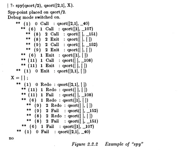
“trace”

Whenitis toomessy toexamine

au

_{the trace list step by step,} we often focus

our

atten-tion on the behavior of specific predicates. Let us put a spy point

on

the predicate $qsort/2$’

inthe program ofExample 2.1.1 and trace theexecution ofan atom qsort$([2,1], X)$ _using

$|?-$ spy(qsort/2), qsort$([2,1], X)$

.

Spy-point placed on $qsort/2$

.

Debug mode switched on.

$**$ ₍₁₎ $0$ Call : qsort$([2,1], -40)$ $**$ _{(6) 1 Call} : qsort_{$([1], -107)$} $**$ _{(8) 2} Call : qsort_{$([], -151)$} $**$ _{(8) 2} Exit : qsort_$([]$, [ ]$)$ $**$ _{(9) 2 Call} : qsort_{$([], -152)$} $**$ _{(9) 2 Exit} : _qsort$([]$, _{[ ]}$)$ $**$ _{(6) 1 Exit : qsort([1], [ ])} $**(11)$ $1$ Call : qsort$([], -108)$ $**(11)$ $1$ Exit : qsort$([]$, [ ]$)$ $**$ _{(1) $0$ Exit : qsort$([2,1], [ ])$} $X=[]$ ; $**$ ₍₁₎ $0$ Redo : qsort$([2,1], [ ])$ $**(11)$ 1 Redo : qsort$([]$, [ ]$)$ $**(11)1$ Fail : qsort$([], -108)$ $**$ _{(6) 1 Redo : qsort([1], [])} $**$ _{(9) 2 Redo : qsort$([]$}, _{[ ]}$)$ $**$ _{(9) 2 Fail : qsort$([], -152)$} $**$ _{(8) 2 Redo : qsort$([]$, [ ]}$)$ $**$ _{(8) 2 Fail : qsort$([], -151)$} $**$ _{(6) 1 Fail : qsort([l], $-107$)} $**$ _{(1) $0$ Fail : qsort$([2,1], -40)$} no

Figure 2.2.2 Example

_of

“spy”

In Section 3, first, atop-down diagnosis algorithm inthe “trace“

manner

is goingtobe

developed for systematizingthe process ofexamining trace lists. Then, atop-down diagnosis

algorithm in the “spy” manner is going to be developed for systematizing the process of

examining specific predicates.

2.3 ProofTree and Search Tree

We can show a diagnosis algorithm using the terminology of “trace list”. However,

it is difficult to formally discuss the properties of the diagnosis algorithm, e.g., soundness

and completeness, using the terminology. So we will give the diagnosis algorithm using the

terminology of “proof tree” and “search tree”.

(1) ProofTree

A proof tree ofan atom $A$ in a

program

$P$ is a tree $T$ whose nodes are labelled with

atoms

as

follows: $T$ is a proof tree of $A$ when $T$ has immediate subtrees $T_{1},$ $T_{2},$ $\ldots,$

$T_{n}$

$(n\geq 0)$ with their root labels $A_{1},$ $A_{2},$

$\ldots,$ $A_{n}$ satisfying the following conditions. The root

label of$T$ is $A,$ $A$ :- $A_{1},$ $A_{2},$

$\ldots,$$A_{n}$

’ is an instance _of

some

_{clause in} $P$, and $T_{1},$ $T_{2},$ $\ldots,$

$T_{n}$

are proof trees of$A_{1},$ $A_{2},$

$\ldots,$ $A_{n}$ in $P$. The clause $A$ :- $A_{1},$ $A_{2},$ $\ldots,$ $A_{n}$

’ _{is said to be used}

at the root of the proof tree $T$, and the atoms $A_{1},$ $A_{2},$

$\ldots,$ $A_{n}$ are caJled child atoms of$A$ in

$T$

.

Example 2.3.1 Anatom qsort([2, 1], [])“ is acomputed solution of atom qsort$([2,1], X)$

153

The child atoms of qsort([2,1],[])” in this proof tree are

partition([l],2,[1], []), qsort$([1], [ ])$, qsort$([]$, [ ]$)$ and append$([], [2], [])$.

The clause used at the root in this proof tree is

qsort([2, 1], []) :- partition([l], 2, [1], []), qsort([l], []), qsort$([]$, []$)$,append$([], [2], [])$.

(2) Proof Subtree

A subtree ofaprooftree $T$ is called aproof subtree of$T$. In particular, aproofsubtree

is called an immediate $p$

roof

subtree of$T$ when

(a) it is properly contained in $T$, and

(b) it is not properly contained in any proof subtree satisfying (a).

The root labels of the immediate proof subtrees of$T$ are child atoms of the root label of$T$

.

Example 2.3.2 The following is an immediate proof subtree of the proof tree of

Exam-ple 2.3.1.

(3) Search Tree

A search tree of an atom sequence $G$ in a program $P$ is a tree $T$ whose nodes are

labelled with atom sequences and whose edges are labelled with substitutions

as

follows: (a) If$G$is an empty atom sequence, $T$is a search tree of$G$ when it is a tree consisting of

only one node labelledwith $\square$

.

(b) If$G$ is a non-empty atom sequence $A,$ $L’$ , let $A_{1}$ :- $L_{1^{y}}$) $A_{2}$ :- $L_{2}’,$

$\ldots,$ $A_{n}$ :- $L_{n}$

“ be all the clauses whose heads are unifiable with $A$, sayby m.g.$u$. $s\theta_{1},$ $\theta_{2},$

$\ldots,$

$\theta_{n}$

.

Let

$T_{1},$ $T_{2},$

$\ldots,$ $T_{n}(n\geq 0)$ be all immediate subtrees of$T$, and $G_{1},$ $G_{2},$ $\ldots,$ $G_{n}$ be their

root labels. $T$ is a search tree of$G$ when the following conditions are satisfied.

b-l $G_{i}$ is ofthe form $(L;, L)\theta_{i}’$

.

The atomsequences $G_{1},$ $G_{2},$

$\ldots,$ $G_{n}$ are caUed child

atom sequences of$G$in$T$

.

Theclause $(A_{i}:- L_{i})\theta$; is said to be used at the root

of the search tree $T$.

b-2 $\theta_{i}$ is the label of the edge from the root nodeof$T$ to the root node of$T_{i}$.

b-3 $T_{i}$ is a search tree of $G_{i}$ in $P$

.

A pathin a search tree from the root to a node labelled with $\square$ is called a

success

path.

A search tree of an atom $A$ in a program $P$ is a search tree of the atom sequence

consisting of only one atom $A$

.

A success path in a search tree of $A$ corresponds to

some

Example 2.3.3 When an atom perm$([2,1], X)$ is executed in the program of Example 2.1.2, it returns only one computed solution perm$([2,1], [2,1])$

.

Its search tree is as below:

perm$([2,1], X)$

$|$ _$\{\}$

perm([l],$Y$),$insert(2, Y, X)$

$|$ _$\{\}$

perm$([], Z)$,insert(l,$Z,$$Y$),$insert(2, Y, X)$

$|$ _{$\{Z\Leftarrow[]\}$}

insert$($1,[],$Y),$$insert(2, Y, X)$

$|$ _{$\{Y\Leftarrow[1]\}$}

insert$(2, [1], X)$

$|$

$\{X\Leftarrow[2,1]\}$

$\square$

The child atom sequence of perm$([2,1], X)$ in the search tree is only

“perm([l],$X$),$insert(2, Y, X)$

.

The clause used at the root in this search treeis

perm$([2,1], X)$ :- perm([l],$Y$), $insert(2, Y, X)$.

(In this example, because the second clause for insert is missed, the search tree is a tree without multiple branching, i.e., a path. But, thisis not acase in general.)

(4) Search Subtree

Let $T$ be a search tree, and $\nu_{1}$ be a nodein$T$ labelled with non-empty atom sequence.

Consider a path $U$ from the node $\nu_{1}$ to a node $\nu_{2}$ in $T$ such that, for every node $\nu$ on the

path other than $\nu_{2}$,

length(v) $\geq length(v_{1})$

holds. (length(v) denotes the number of atoms in the label of$\nu.$) Then, the path, which is

constructed by neglecting last length$(\nu_{1})-1$ atoms in the label of every node on the path

$U$, is called a subdeduction at the node $\nu_{1}$ in $T$.

Let $\nu$ be a node in a search tree $T$, and $U_{1},$ $U_{2},$ $\ldots,$

$U_{h}$ be all subdeductions at $\nu$ in

$T$, that are not properly contained in any subdeduction at $\nu$ in $T$

.

Then, the tree, which is

constructed by putting the paths $U_{1},$ $U_{2},$ $\ldots,$

$U_{h}$ together, is called a search subtree of$T$ at

$\nu$

.

Let $T_{1}$ and $T_{2}$ be search subtrees of$T$ at $u_{1}$ and $u_{2}$, respectively. Then, $T_{2}$ is said to be

properly contained in $T_{1}$ when $T_{2}$ is a search subtree of$T_{1}$ at some node $u$ other than the

root nodein $T_{1}$, and the node $u$ corresponds to $u_{2}$ in $T$

.

Note that the root label ofa search

subtree is always one atom, and asearch subtree with rootlabel $A$’ is asearch tree of $u_{A’}$ .

In particular, a search subtree of$T$ is caUed

an

immediate search subtree of$T$ when

(a) it is properly contained in $T$, and

1

$5_{c/}^{\iota:}$

Example

_2.3.4

The tree belowis an immediatesearch subtree of the search tfeeof Example 2.3.3. (Because the original search tree does not have a multiple branching, neither does this immediate search subtree. But, this is not a case in general, either.)

perm$([1], Y)$

$|$ _$\{\}$

perm$([], Z),$$insert(1, Z, Y)$

$|$ _{$\{Z\Leftarrow[]\}$}

insert$(1, [], Y)$

$|$ _{$\{Y\Leftarrow[1]\}$}

$\square$

The tree below is the part of the search tree which consists of the nodes corresponding to those in the search subtree above.

perm([l],$Y$),$insert(2, Y, X)$

$|$ _$\{\}$

perm$([], Z),$$insert(1, Z, Y),$$insert(2, Y, X)$

$|$ _{$\{Z\Leftarrow[]\}$}

insert(l, [],$Y$),$insert(2, Y, X)$

$|$ _{$\{Y\Leftarrow[1]\}$}

insert$(2, [1], X)$

3. Top-down Zooming Diagnosis of Logic Programs

In this section, we will first present two kinds of unexpected execution-results. Next, we will presentatop-downdiagnosisalgorithm in the “trace“ ,.nnel. Then,wewill improve

the top-down diagnosis algorithm in the (spy’ manner.

3.1 Unexpected Success and Unexpected Failure

(1) Unexpected Success (Incorrect Solution)

Suppose that the

execution

of an atom $A$ has succeeded with computed solution $A\theta$

.

If$A\theta$ is invalid in our intended interpretation _$M,$ $A\theta$ is said to have succeeded unexpectedly w.r.$t$. $M$

.

Example 3.1.1 Anatom qsort$([2,1], X)$ intheprogram ofExample 2.1.1 has acomputed solution qsort([2, 1], [ ]). But it is invahd w.r.$t$. our intention. Hence, the success of atom

(2) Query for Invalid Instances

Toexamine whether anatom$A$hassucceeded unexpectedlyornot, ourdiagnoser issues

a query as follows :

“Is some instanceof$A$ false¿‘

The answer for this query is either “Yes” or “No“.

“Yes“ : The atom $A$ is invalid, hence, it has succeeded unexpectedly.

“No”: The atom $A$ is valid, hence, it is an intended solution.

Example 3.1.2 In Example 3.1.1, our diagnoser asks a query as follows:

“Is some instance of qsort([2, 1], [ ]) false?”

The human programmer (or oracle) answers “Yes”, hence the

success

of qsort$([2,1], [])$ is an

unexpected one.

(3) Unexpected Failure (Missing Solution)

Suppose that the execution ofan atom $A$ has failed after returning several (possibly

zero) computed solutions that are all valid in our intended interpretation $M$. If the atom $A$

has some missed solution, the atom $A$ is said to have

failed

unexpectedlyw.r.$t$

.

$M$.

Example 3.1.3 The execution of atom perm$([2,1], X)$ in the program of Example 2.1.2

fails after returning only one computed solution perm$([2,1], [2,1])$ , which is valid in our

intention. But the atom has a missed solution perm$([2,1], [1,2])$ . Hence, the last failure

of atom perm$([2,1], X)$ is an unexpected one.

(4) Query for Valid Instances

Suppose that the execution of an atom $A$ has failed after returning several (possibly

zero) computed solutions, which has been already confirmed to be validin ourintended

inter-pretation. To examine whether the execution has failed unexpectedly or not after obtaining

these computed solutions, our diagnoser issues a query as follows: “Is some other instance of $A$ true?”

The answer for these queries is either “Yes” or “No”.

“Yes“: The atom $A$ has some missed solution, hence,it has failed unexpectedly.

“No“ : The atom $A$ has all intended solutions.

Example

_3.1.4

Suppose that

au

computed solutions of an atom perm$([2,1], X)$ in the

program of Example 2.1.2 have been confirmed to be correct w.r.$t$

.

our intention. Then our

diagnoser asks a query as follows:

“Is some other instance ofperm$([2,1], X)$ true?”

The human programmer (or oracle) answers “Yes“. Hence the last failure of perm$([2,1], X)$

(with only one computed solution perm$([2,1],$ $[2,1])$) is an _unexpected one.

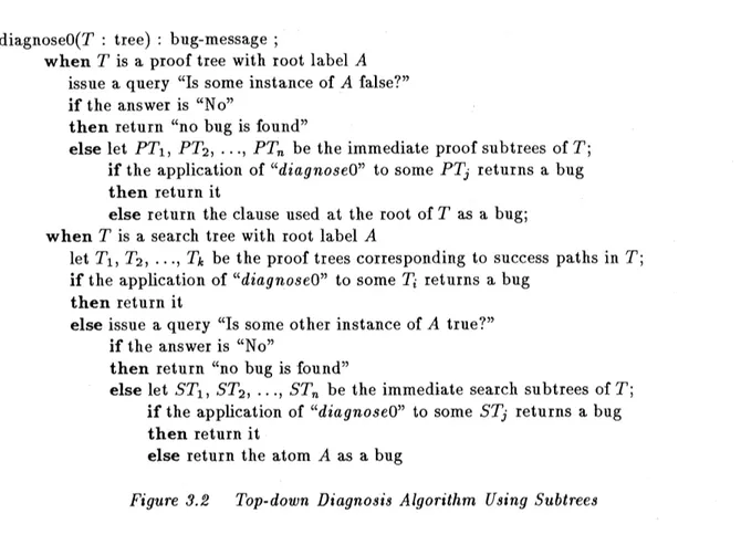
3.2 Top-down Diagnosis Algorithm

The top-down diagnosis algorithm “diagnose0” receives a tree (either

a

proof tree or a search tree ofan atom), and returns a definite clause instance, an atom, or a

message

“no

1

$5^{\backslash }$

,

diagnose0(T : tree) : bug-message ;

when $T$ is a prooftree with root label $A$

issue a query “Is some instance of$A$ false?”

if the

answer

is “No”

then return “no bug is found”

else let $PT_{1},$ $PT_{2},$ _$\ldots,$ $PT_{n}$ be the immediate proof subtrees of$T$;

if the application of “diagnose0” to some $PT_{j}$ returns a bug

then return it

else return the dause used at the root of$T$ as a bug;

when $T$ is a search tree with root label $A$

let $T_{1},$ $T_{2},$ $\ldots,$

$T_{k}$ be the proof trees corresponding to success paths in $T$; ifthe application of “diagnose0” to some $T_{i}$ returns a bug

then return it

else issue a query “Is some other instanceof $A$ true?”

if the answer is “No”

then return “no bug is found” else let $ST_{1},$ $ST_{2},$

$\ldots,$ $ST_{n}$ be the immediate search subtrees of

$T$;

if the application of “diagnose0” to some $ST_{j}$ returns a bug

then return it

else return the atom $A$ as a bug

Figure 3.2 Top-down Diagnosis Algorithm Using Subtrees

The following theorem holds for this algorithm. (See [7] for this proof.) Theorem 3.2 (soundness and completeness

_of

the top-down diagnosis algorithm)

Let $P$ be a terminating program, $M$ be an intended interpretation, and $T$ be a tree

(either a proof tree or a search tree) ofan atom A. Th$e$ execution-result of the atom $A$ in $P$

is incorrect $w.r.t$

.

$M$, ifan$d$ only if ”diagnose0“ applied to $T$ retu_$rns$ either a

wrong

clause

instance or an uncovered atom $w.r.t$. $M$

.

In the following examples, an “answer database” accumulates answers to previous queries in order to partly mechanize the oracle answers. A new query is first posed to the “answer database”. Only if the “answer database” fails to answer it, a query is issued to the programmer (or an oracle), and the answer is added to the “answer database”. (See Shapiro [10].)

Example 3.2.1 Let us diagnose an atom qsort$([2,1], X)$ in the program of Example 2.1.1.

In the following, “diagnose0” takes the root label of each tree as an argument instead ofthe

$t$ree itself. (See section 4.1 for its implementation.)

$|?-$ diagnose0(qsort([2, 1],$X$)).

Is some instance of qsort([2, 1], []) false? yes.

Is some instance of partition([l], 2, [1], []) false? no.

Is some instance of qsort([l],[]) false? yes.

Is some instance of partition([], 1, [], []) false? no.

Is

some

instance of qsort$([]$, []$)$ false? no.

Is some instance of append$([], [1], [])$ false? yes.

yes

Example 3.2.2 Let us diagnose an atom perm$([2,1], X)$ in the program of Example 2.1.2.

$|?-$ diagnose0(perm([2, 1],$X$)).

Is some instance ofperm$([2,1], [2,1])$ false? no.

Is some other instance ofperm$([2,1], -47)$ true? yes.

Is some instance of perm([l], [1]) false? no.

Is some other instance of perm([l],$-319$) true? no.

Is some instance ofinsert$(2, [1], [2,1])$ false? no.

Is some other instance ofinsert$(2, [1], -47)$ true? yes.

%%% Uncovered Atom %%% insert$(2, [1], -47)$

X $=-47$

yes

3.3 Top-down Zooming Diagnosis Algorithm

During the the top-down diagnosis, our diagnoser issues several queries for human

programmers (or oracles). All these queries are issued about instances of atoms, whose

predicate may change query by query. The human programmers must change his attention

according to the predicates of atoms. Instead, we can change the order of queries to issue

the queries about atoms with the same predicate continually so that the burden of human

programmers is lightened. This change of the order also makes it possible to quickly narrow

down the location containing a bug.

(1) Immediate Recursion Subtree in Proof Trees

Let $T$ be a proof tree in a program $P$ whose root label is an atom $A$ with predicate $p$. A proof subtree in $T$ is called a recursion proof subtree of$T$ when its root label is with

predicate$p$. In particular, aproof subtree in $T$is called an immediate recursion proof subtree

when

(a) it is properly contained in $T$,

(b) the root label of the proof subtree is with predicate$p$, and

(c) it is not properly contained in any proofsubtree satisfying (a) and (b).

Example 3.3.1 In the proof tree of Example 2.3.1, the atom qsort([2, 1], [ ]) has only two immediate recursion proof subtrees with roots qsort([l], [ ]) and qsort$([]$,[ ]$)$.

(2) Immediate Recursion Subtree in Search Trees

Let $T$ be a search tree in a program $P$ whose root label is an atom $A$ with predicate $p$. A search subtree in $T$ is called a recursion search subtreeof$T$ when its root label is with

predicate $p$. In particular, a search subtree in $T$ is called an immediate recursion search

subtree when

(a) it is properly contained in $T$,

(b) the root label is with predicate$p$, and

(c) it is not properly contained in any search subtree satisfying (a) and (b).

Example 3.3.2 In the search tree of Example 2.3.3, the atom perm$([2,1], X)$ has only

I.59

(3) A Top-down Zooming Diagnosis Algorithm Using Recursion Subtrees

The top-downzoomingdiagnosis algorithm usingrecursion subtrees is almost the same as the previous top-down diagnosis algorithm “diagnose0” except that it works with aids of a subprocedure “zooming“, which receives a tree and returns a subtree for diagnosis by searching for recursion subtrees.

diagnose(T : tree) : bug-message ;

if the application of “zooming” to $T$ does not return a tree

then return “no bug is found”

else let $T’$ be the tree returned by “zooming“ when$T’$ is a proof tree with root label $A$

let $PT_{1},$ $PT_{2},$ _$\ldots,$ $PT_{n}$ be the immediate proof subtrees of$T’$;

ifthe application of “diagnose” to some $PT_{j}$ returns a tree

then return it

else return the dause used at the root of$T’$ as a bug; when $T’$ is a search tree with root label $A$

let $ST_{1},$ $ST_{2},$

$\ldots,$ $ST_{n}$ be the immediate search subtrees of$T’$;

ifthe application of “diagnose” tosome $ST_{j}$ returns a bug

then return it

else return the atom $A$ as a bug

zooming(T : tree) : tree ;

when $T$ is a proof tree with root label$A$

issue a query “Is some instance of$A$ false?”

ifthe answer is “No”

then return “no tree is found”

elselet $PT_{1},$ $PT_{2},$ _$\ldots,$ $PT_{n}$ be the immediate recursion proofsubtrees of$T$;

if the application of “zooming” to some $PT_{j}$ returns a tree

then return it

else return $T$

when $T$ is a search tree with root label $A$

let $T_{1},$ $T_{2},$ $\ldots,$

$T_{k}$ be the proof trees corresponding to success paths in $T$;

ifthe application of “_{zooming” to} some $T_{i}$ returns a tree

then return it

else issue a query “Is some other instance of$A$ true?”

ifthe answer is “No”

then return “no tree is found” else let $ST_{1},$ $ST_{2},$

$\ldots,$ $ST_{n}$ be the immediate recursion search subtrees of$T$;

ifthe application of “zooming” to

some

$ST_{j}$ returns a tree

then returnit

else return $T$

Figure 3.3 Top-down Zooming Diagnosis Algorithm Using Recursion Subtrees

Roughly speaking, the top-down zooming diagnosis algorithm identifies the subtrees

containing a bug by changing its attention in the following two different ways by turns.

(a) One way is to

narrow

down to immediate recursion subtrees quickly by changing

recursion subtree such that the execution-result ofits root label is incorrect but the execution-result of root labelofevery immediaterecursion subtree is correct w.r.$t$

.

$M$. (b) The other way isto narrow down to the immediate subtrees slowly in thesame way as “diagnose0“. “diagnose“ _{above proceedsinthe same way as “diagnose0” after making}

use of “zooming” first.

Thefollowing theorem holds for this algorithm. (See [7] for this proof.)

Theorem 3.3 (soundness and completeness

_of

the top-down zooming diagnosis algorithm)

Let $P$ be a termin ating program, $M$ be an inten$ded$ interpretation, an$dT$ be a tree

(either a proof tree or a search $tree$) ofan a tom A. When the exec$u$tion-res$ult$ of the atom

$A$ in $P$is incorrect _$w.r.t$

.

$M$, ifand onlyif “diagnose“ appli$ed$ to$Tre$tu$rns$ either a wrong

$cl$ause instan_$ce$ or _$an$ uncovered atom _$w.r.t$

.

$M$

.

Example 3.3.3 Let us diagnose the atom qsort$([2,1], X)$ in the program ofExample 2.1.1 by this top-down zooming diagnosis.

$|?-$ diagnose(qsort([2, 1],$X$)).

Is some instance of qsort([2, 1], []) false? yes.

Is

some

instance of qsort([l], []) false? yes.

Is some instance of qsort$([]$,[]$)$ false? no.

Is some instance of partition([],1,[], [ ]) false? no.

Is

some

instance of append$([], [1], [])$ false? yes.

%%% Wrong Clause Instance %%% append$([], [1], [])$

yes

Example

_3.3.4

Let us diagnose the atom perm$([2,1], X)$ in the program of Example 2.1.2 by this top-down zooming diagnosis.

$|?-$ diagnose(perm([2, 1],$X$)).

Is

some

instance ofperm$([2,1], [2,1])$ false?

no.

Is some other instance ofperm$([2,1],-47)t$rue? yes.

Is some instance of perm([l], [1]) false? no.

Is

some

other instanceof perm([l],$-319$) true? no.

Is

some

instance ofinsert$(2, [1], [2,1])$ false? no.

Is some other instance of$\iota’nsert(2, [1], -47)$ true? yes.

%%% Uncovered Atom %%% insert$(2, [1],-47)$

X $=-47$

yes

4. Implementation of the Top-down Zooming

Diagnosis

Algorithm

In this section, we will show a brief outline of an implementation of the top-down

zooming diagnosis algorithm.

4.1 Consideration on Space Efficiency

We

assume

that all the trees used in the diagnosis ofSection3.3 are recorded ina “tree database“. They are used somehow for processing proof trees and search trees, which are

passed as arguments of “diagnose“ and “zooming”. However, recording all the trees is very

16]

(a) “diagnose” recurses with an immediate subtree,

(b) “zooming”

recurses

with some tree, either an immediate recursion subtree or a proof tree corresponding to success path, or

(c) “zooming” issues a query about the root label of the tree.

So, ifwe can obtaintheroot labels ofanyimmediate subtree, anyimmediate recursion

subtree, and any proof tree corresponding to success path somehow, it is enough for the diagnosis. Let $A$ be a root label of a tree.

The root label of its immediate subtree are obtained from $A$ by repeating only the

top-level ofthe computation using the root labels of trees as follows: (a) When $A$ is a root label of a proof tree $PT$, let $A_{1},$ $A_{2},$

$\ldots,$ $A_{n}$ be the root labels of

all immediate proof subtrees of $PT$. Then there is a clause $B:- B_{1},$$B_{2},$

$\ldots,$$B_{n}$

“ _in

$P$ and a substitution $\theta$ such that _{$A_{i}\equiv B_{i}\theta(1\leq i\leq n)$} and $A\equiv B\theta$ hold. On the

other hand, if thereis aclause $B:- B_{1},$$B_{2},$ $\ldots,$$B_{n}$

“ _{in $P$and a substitution} $\theta$ such that

$A_{1}\equiv B_{1}\theta,$ $A_{2}\equiv B_{2}\theta,$

$\ldots,$ $A_{n}\equiv B_{n}\theta$hold for

some

root labels

$A_{1},$ $A_{2},$

$\ldots,$ $A_{n}$ of proof

trees in the “tree database”, then $B\theta$ should succeed in $P$ using the dause instance $(B:- B_{1}, B_{2}, \ldots, B_{n})\theta$’ in $P$. Hence, we may conclude that there is aprooftree for $B\theta$

in the “tree database” such that the root labels of all its immediate proof subtrees are

the atoms $A_{1},$ $A_{2},$

$\ldots,$ $A_{n}$

.

(b) When $A$is a rootlabel ofasearch tree $ST$, let $A’$ be aroot labelofanimmediate search subtree of ST. Then there is a clauseinstance $H:- A_{1},$$A_{2},$

$\ldots,$$A_{n}$ such that the head

is unifiable with $A$, say by $\sigma$, and $A_{i}\sigma\theta$ is equal to $A$‘ for some computed solution $(A_{1}, A_{2}, \ldots, A_{i-1})\sigma\theta$ of $(A_{1}, A_{2}, \ldots, A_{i-1})\sigma$ $(1\leq i\leq n)$

.

On the other hand, all the

atoms constructed by such a way are the root labels of immediate search subtrees of

ST.

The root labels of immediate recursion subtrees are obtained by constructing the root labels of immediate subtrees recursively.

The root labels of proof trees corresponding to

success

paths ofasearch tree for $A$ are

obtained with less time (in compensation for the spacefor recording), if we record them in

the structure which associates $A$ to the root labels of such proof trees.

Hence, the root labels of subtrees are all obtained by using the clauses in $P$ and the

recorded root labels of trees.

Now, we do not need all the information in the trees. The information we record in

the “tree database“ is only

(a) the root labelsof proof trees, and

(b) the pairs of the root label of a search tree, and the sequence of the root labels ofits

proof trees corresponding to success paths.

(Hence, it is more appropriate to $caU$ it a “label database”.) Due to this implementation

method, the arguments of “diagnose” and “zooming” are now not trees but root labels of the trees.

4.2 Consideration on Time Efficiency

Even if we have employed a space-efficient representation above, the space required

for recording them is stiu large. We can reduce the necessary space at each instance by

recording only some root labels ofthe tree which is immediately necessary for the present,

and by recomputing another root labels which will become necessary later. In the top-down

zooming diagnosis, we do not need to immediately search root labels of trees other than

subtrees relevant for the present. The computation of the root labels of trees other than

recursion subtrees is done afterwards ifnecessary.

If we have employed such an implementation method for reducing space at each

in-stance, it may require much more time due to the recomputation, i.e., some goals might

have to be re-executed again and again during the diagnosis. However, note that the atoms

appearing in the re-execution are only those appearing in the execution before. Hence, we

canimprove the time-efficiency byutilizing the root labels of prooftrees,that areused before for the diagnosis, during each re-execution to avoid

some

ofthe recomputation.

4.3 Consideration on Query

As was already used in the previous examples, an “answer database“ accumulates

answers to previous queries in order to partly mechanize the oracle answers. A new query

is first posed to the “answer database“. Only if the “answer database“ fails to answer it,

the query is asked to a programmer (or an oracle), and the

answer

is added to the “answer

database“. (See Shapiro [10].)

(1) Collective Queries

The queries can be improved to be more natural for human programmers in several points. For example, it is more natural to ask

“Is some instance of$A$ true¿‘

instead of “Is some other instance of $A$ true?” when $A$ has failed without returning any

computed solution. It is also more natural to ask “Is $A$ true¿‘

ccIs $A$false¿‘

when the atom $A$ in queries are ground.

In additionto sucheasy improvements, it ismorecomfortable for humanprogrammerto

answer severalrelated questions atonestroke. Such queries reduce the number ofanswersthe

programmer must typein. For example,in the diagnosis for unexpected success, the queries

for the root labels ofevery immediate recursion subtrees (or every immediate subtrees) can

be issued together. Similarly, in thediagnosis for unexpected failure, the queries for the root labels of proof trees corresponding to success paths can be issued together.

Example

_4.3.1

Let us diagnose the atom qsort$([2;1], X)$ in the

program

of Example 2.1.1

by issuing several queries together.

$|?-$ diagnose(qsort([2, 1],$X$)).

Is some instance of thefollowing atoms false?

1 : qsort([2, 1], []) Which? 1. 1 : qsort([l], [ ])

2 : qsort$([]$,[]$)$ Which? 1.

1 : qsort$([]$,[]$)$ Which? no.

1 :

part\’ition([],

1,[], [])

2 : append$([], [1], [])$ Which? 2.

%%% Wrong Clause Instance %%% append$([], [1], [])$

163

Example

_4.3.2

Let us diagnose the atom perm$([2,1], X)$ in the program of Example 2.1.2

in the same way.

$|?-$ diagnose(perm([2, 1],$X$)).

Is some instance of the following atoms false?

1 : perm$([2,1], [2,1])$ Which? no.

Is some other instance ofperm$([2,1], -47)$ true? yes.

1 : perm([l], [1]) Which? no.

Is some other instance of perm([l],$-319$) true? no.

1 : insert$(2, [1], [2,1])$ Which? no.

Is some otherinstance ofinsert$(2, [1], -47)$ true? yes.

%%% Uncovered Atom %%% insert$(2, [1],-47)$

X $=-47$

yes

(2) Query for Instances of Missed Solutions

Aswas adopted by Shapiro [10] and Lloyd [6], we can enjoyboth the timeefficiency and

the spaceefficiency, ifan oraclecangive a suitableinstantiation of variablesto thediagnoser.

Suppose that the diagnoser is modified to ask the oracle to give a missed solution when an

oracle has given an answer “Yes” for a query “Issome other instance of$A$ true?”. If such a

missed solutionis given, the number of queries decreases in some cases, because the number of immediate search subtrees to be diagnoses decreases.

Example

_4.3.3

Let sort be a predicate defined by

sort(L,N) :-perm(L,N), ordered(N).

perm$([],[ ])$

.

perm$([X|L],N)$ :-perm(L,M), insert$(X,M,N)$. insert$(X,M,[X|M])$.

insert$(X,[Y|M],[Y|N])$ :- insert$(X,M,N)$

.

lt misses the program of the predicate ordered. The diagnosis proceeds as below if the previous algorithm is used.

$|?-$ diagnose(sort([2,3,1],$X$)).

Is some instance of sort$([2,3,1],-55)$ true? yes.

Is some instance of perm$([2,3,1], [2,3,1])$ false? no.

Is

some

instance ofperm$([2,3,1], [3,2,1])$ false? no.

Is some instance ofperm$([2,3,1], [3,1,2])$ false? no.

Is some instance ofperm$([2,3,1], [2,1,3])$ false? no.

Is some instance ofperm$([2,3,1], [1,2,3])$ false? no.

Is some instance of perm$([2,3,1], [1,3,2])$ false? no.

Is

some

other instance of perm([2, 3, 1], -S5) true? no.

Is some instance of ordered([2, 3, 1]) true? no.

Is some instance ofordered([3, 2, 1]) true? no.

Is some instance ofordered([3, 1, 2]) true? no.

Is

some

instance ofordered([2, 1, 3]) true? no.

Is some instance of ordered([l, 2, 3]) true? yes.

X $=[1,2,3]$

yes

If thediagnoser is modifiedas given in this section, thediagnosis process is as shown below.

$|?-$ diagnose(sort([2,3, 1],$X$)).

Is some instance ofsort$([2,3,1], -55)t$rue? yes.

What is the correct instance

_of-55

? [1,2,3].

Is some instance ofperm$([2,3,1], [1,2,3])$ false? no.

Is some instance of ordered([l, 2, 3]) true? yes.

%%% Uncovered Atom %%% ordered([l, 2, 3])

X $=[1,2,3]$

yes

When a programmer knows that there are some missed solutions, $he/she$ probably

knows some ofthe missed solutions. Of course, $he/she$ may refuse to give such an instance

if$he/she$ thinks it troublesome to give a concrete true instance. We are not sure, however,

which imposes less burden on the

programmers

in general. It dependson the characteristics

ofprograms.

(3) Oracle Answer “Unknown”

So far, wehave assumed that the oracle returnsadefinite answer “Yes” or “No”. When the oracleis a human programmer, however, $he/she$may want togive an answer “Unknown” occasionally. We can modify the diagnoser so as to accept such an answer.

Recall the differences between the top-down diagnosis and the top-down zooming

di-agnosis. The latterwas in the same way as the former except that the recursion subtreesare

diagnosed in the preference to the top-down manner by zooming.

Suppose that the answer “Unknown” is returned. We may continue the diagnosis by preference for the other subtrees in the same way as zooming. Ifthe definite answer ofthe rootnode of this treeisneeded finally,the diagnoser asksagaintoreturn thereservedanswer.

5. Discussion

Debuggingoflogicprogramshas been studied by several researchers intensively. Shapiro

[10] said that

program

debugging is composed ofprogram diagnosis, the process ofiinding a

bug, and program correction, the process offixing the bug. In this paper wehave discussed

the program diagnosis.

We have attributed incorrectness ofprograms to two bugs, wrong clause instance and uncovered atom in the same way as Shapiro [10], Lloyd [6], et al. However, wrong clause

instances and uncovered atomsin our definitions are slightly different from those in Shapiro

[10] or Lloyd’s definitions [6]. For example, in the definition of a wrong clause instance by Lloyd [6], the condition (a) in Definition 2.1.1 is replaced with the following:

(a) the atom $A$ is unsatisfiable in $M$, i.e.,

au

groundinstances of$A$ are false in $M$, and“

In the definition ofan uncovered atom by Lloyd [6], an atom $A$ is cffied an uncovered atom

when

16.5

$arrow(b)$ for any clause $B$ :- $L$’ in $P$ whose head $B$ is unifiable with $A$, say by an m.g.$u$. $\theta,$ $L\theta$ is unsatisfiable in $M$, i.e., a1I ground instance of$L\theta$ arefalse in $M$

.

Theorem 2.1 is the same as Proposition 3 in Lloyd [6] p.6. These differences do not affect the proof of this theorem.

Our definition of correctness is stronger than that of Lloyd [6]. Our definition implies that a program $P$ is correct w.r.$t$

.

an intended Herbrand model $M$ if and only if $M$ is the

least Herbrand model of completion $P^{*}$, while his definition is that a program $P$ is correct

w.r.$t$. an intended model $M$ if and onlyif$M$ is a model of completion $P^{*}$. Hence, for proving

Theorem 2.1, we needed an additional condition “terminating”.

In additionto thesesubtle differences of definitions, our diagnosesalgorithm isdifferent from theirs in several respects.

(1) Our diagnosis algorithm is basically top-down.

Shapiro’s algorithm [10] for unexpected success (incorrect solution) is in the

bottom-up manner, while that for unexpected failure (missing solution) is in the top-down manner.

There is no inherent reason to stick to the bottom-upmanner. In fact, Lloyd [6] showed the top-down algorithm for unexpected success.

Similarly to Lloyd [6], our diagnosis algorithm is basicaly top-down. Fornon-recursive

predicates, our approach issues queries in the usual top-down manner so that the

program-mers can locate bugs more quickly than the single stepping bottom-up diagnoser in general.

(2) Our diagnosis algorithmjust needs answer “Yes” or “No”.

Though our algorithm can accelerates the diagnosis by answering concrete instances

(see Section 4.3), it needs just answer “Yes” or “No” in general due to the utilization of

the previous result of program execution. In both Shapiro [10] and Lloyd [6], the diagnosis

requests an oracle to instantiate variables to suitable forms, because of their definitions of

wrong clause instances and uncovered atoms detected by their diagnosis algorithms.

Of course, recording all the trees is very space-consuming. We can reduce the

neces-sary space at each instance by recording only the parts of the trees which are immediately

necessaryfor the present, and by recomputingthe parts which willbenecessarylater.

More-over we do not need all the information in such parts of the trees (see Section 4.1). For

example, in the top-down zooming diagnosis, we do not need ‘_$0$ immediately search atoms

other than recursions so that the diagnoser needs to record only the relevant recursions, though such reduction ofspace may be inferior in thetime efficiency due to the overhead for

recomputation.

(3) Our diagnosis algorithm issues queries for the same predicate continually.

In general, it is easier and more natural for human programmers to answer queries for

the same predicates continually. For recursive predicates, our approach jumps and omits some intermediate atoms with different predicates so that the queries for atoms with the same predicate are issued to the programmers continually. (Our concern is close to that of Eisenstadt [1].)

Moreover, such queries sometimes identify the segment containing bugs more quickly. Plaisted [9] showed a buglocation algorithm more efficient than Shapiro’s original algorithm.

His method selects nodes of trees (either prooftrees or search trees), called cutoffs, in such a way that theexecution time ofeach node distributes asuniformlyw.r.$t$. the computation time as possible with some average interval, and roughly identify subcomputation containing a bug first, then apply his methods recursively to the subcomputation. Though our approach is not eager in uniformly distributing nodes for queries, the similar effect is obtained by leaping to immediate recursion subtrees.

Several problems still remain. One is that we have restricted our target program to

terminating one. (See Kanamori[4] for detection of Prolog program termination.) Another

problem is that we have restricted our target programming language to pure Prolog. The extra-logical control symbols like cut(!) and the predicates with side-effectslike “assert” and

“retract” are neglected. (These restrictions can be relaxed to a certain extent.)

6. Conclusions

We have shown a framework for top-down zooming diagnosis of logic programs. This method is an element ofour system for analysis of Prolog programs $Argus/A$ under

devel-opment $[2],[3],[4]$.

Acknowledgements

Our analysissystem $Argus/A$ under developmentisa subproject of the Fifth Generation Computer System (FGCS) “Intelligent Programming System”. The authors would hke to

thank Dr. K. Fuchi (Director ofICOT) for the opportunity of doing this research, and Dr. K. Furukawa (Vice Director of ICOT), Dr. T. Yokoi (Former Vice Director of ICOT) and

Dr. H. Ito (Chiefof

ICOT

3rd Lab.) for their advice and encouragement.

References

[1] Eisenstadt,E., “Retrospective Zooming : A Knowledge Based Tracing and Debugging

Methodology for Logic Programming”, Proc. of 9th International Joint Conference on

Artificial Intelligence, pp.717-719, Los Angeles 1985.

[2] Kanamori,T. and T.Kawamura, “Analyzing Success Patterns of Logic Programs by Abstract Hybrid Interpretation“, ICOT Technical Report TR-279, 1987.

[3] Kanamori,T., K.Horiuchi and T.Kawamura, “Detecting Functionality of Logic

Pro-grams Based on Abstract Hybrid Interpretation’, to appear, ICOT Technical Report,

1987.

[4] Kanamori,T.,T.Kawamuraand K.Horiuchi, “Detecting TerminationofLogic Programs

Based on Abstract Hybrid Interpretation”, to appear, ICOT Technical Report, 1987. [5] Lloyd, J. W., “Foundation of Logic Programming”, Springer-Verlag, 1984.

[6] Lloyd, J. W., “Declarative Program Diagnosis”, Technical Report 86/3, Department of Computer Science, University of Melbourne, 1986.

[7] Maeji,M. and T.Kanamori, “Top-down Zooming Diagnosis ofLogic Programs”, ICOT Technical Report TR-290, 1987.

[8] Pereira,L.M., “Rational Debugging in Logic Programming“, Proc. of 3rd International Conference on Logic Programming, pp.203-210, 1986.

[9] Plaisted,D., “An Efficient Bug Location Algorithm”, Proc. of 2nd International Logic

Programming Conference, pp.151-157, 1984.

[10] Shapiro,E.Y., “Algorithmic Program Diagnosis”, Conf. Rec. of the 9th ACM Sympo-sium on Principles of Programming Languages, pp.299-308, 1984.