Japanese Association for Mathematical Sociology
Can the Signaling Game Serve as a Model of
Statistical Discrimination in Hiring?
Kunihiro Kimura (Tohoku University)
Abstract
Some scholars argue that Spenceʼs signaling game with an index may serve as a model of statistical discrimination in hiring processes. This would then explain that both mean education level and mean wage are greater for men than for women in industrialized societies. To examine the validity of this conjecture, I formulated a generalized version of the game. In this version, I assumed that the educational level is a signal of productivity while the gender is an index of productivity. I then followed the refinement procedure of Perfect Bayesian Equilibria to eliminate unreasonable outcomes. My analysis reveals that an anomaly is derived from the separating equilibrium that survives the Intuitive Criterion in the procedure: the mean wage for men would be equivalent to that for women. As the employer is assumed to know that the educational cost for women is greater than that for men, he or she would believe that women with a lower level of education have the same productivity as men with a higher level of education. Therefore, the employer would offer the same wage for the men and the women. I also examined other classes of equilibria and alternative assumptions.
Keywords
gender gaps in education and wage; perfect Bayesian equilibrium; separating equilibrium; game theory.
Review History
Received April 1, 2019/Accepted August 9, 2019
1
The Gender Gaps in Education and Wage
In most of industrialized societies, we have observed the gender gap in education as well as that in wage (or more generally, in pay). On the one hand, the mean educational level for men have long been greater than that for women, although the growth in female participation rate in tertiary education among younger cohorts contributed to the reduction or even reversal of the gender gap in many OECD member countries in recent years (Vincent-Lancrin. 2008; OECD 2016:29). On the other hand, the mean (or median) wage for men is greater than that for women: the gender wage gap indicator1) for 24 OECD member countries in 2015 ranges from 4.7 (Belgium) to 37.2 (Korea)
Let us take a closer look at the data from Japan as one of the countries that have exhibited greater gender gaps. Figure 1 shows the advancement rate to higher education by gender. Even in 2018, menʼs advancement rate to university is greater than womenʼs. The difference is equal to 6.2 percentage points. If we include those who entered junior colleges, womenʼs rate is 1.0 percentage greater than menʼs. But junior colleges provide only short time, that is, two (or sometimes three) year higher education.
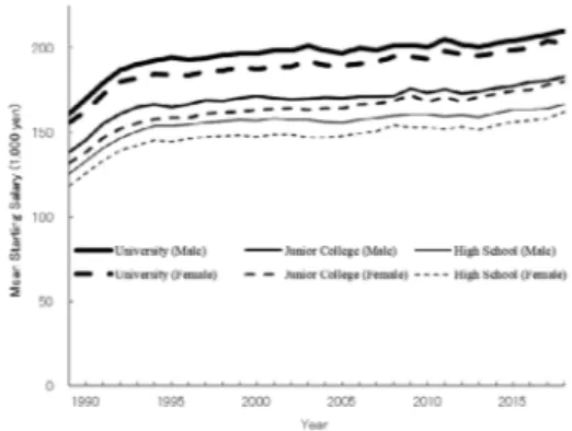
Figure 2 shows the mean starting salaries for ordinary employees who got jobs fresh from school.2) For every year, we can see that although the higher level of education contributes to
the higher amount of the mean starting salary regardless of gender, the gap in salary persists even for men and women of the same education. For example, in 2018, the mean for male university graduates is 210 thousand yen while that for the female counterpart is 203 thousand yen; in the same year, the mean for male high-school graduates is 167 thousand yen while that for the female counterpart is 162 thousand yen.
Figure 1 Advancement Rates to University and Junior
College by Gender in Japan, 1955-2018.
Source: School Basic Survey, MEXT (Ministry of Education, Culture, Sports, Science and Technology), Japan. (Retrieved from Statistics Bureau, Ministry of Internal Affairs and Communications, Japan (n.d.) “e-Stat: Portal Site of Official Statistics of Japan.”)
Figure 2 Mean Starting Salary by Education and Gender in Japan, 1989-2018.
Source: Basic Survey on Wage Structure, Ministry of Health, Labour and Welfare, Japan. (Retrieved from Statistics Bureau, Ministry of Internal Affairs and Communications, Japan (n.d.) “e-Stat: Portal Site of Official Statistics of Japan.”)
Theory of statistical discrimination seems promising in explaining both gender gaps in industrial societies. In the followings, I will review literature on signaling games as a model of statistical discrimination (Section 2). Based on the review, I will formulate a generalized version of Spenceʼs (1974a) signaling game with an index, and follow the procedure of refinements of Perfect Bayesian Equilibria to eliminate unreasonable outcomes (Section 3). For the separating equilibrium that survived the procedure, however, we can find an anomaly or a curious consequence. Although the mean educational level for men is greater than that for women, the mean wage for men would be equivalent to that for women. I will also examine other four equilibria to show that our model may succeed in predicting the gender gap in education but it fails to explain the gender gap in wage (Section 4). Finally, for the development of a more appropriate model of statistical discrimination, I will discuss the process of the employerʼs belief formation, and an alternative assumption of gender-differentiated distribution of productivity (Section 5).
2
Statistical Discrimination and Signaling Games
Decision-makers such as employers and college admission officers have to decide placement of applicants where gaining relevant information of the applicants is excessive. They may rely on statistical reasoning using an observable characteristic as a proxy for the relevant but unobservable characteristic. When this reasoning entails a discriminatory action against members of a targeted group (or groups), we shall call it statistical discrimination (Fang and Moro 2011:134; Phelps 1972).
Although both statistical discrimination theory and taste-based discrimination theory (Becker 1954) emphasize rationality of discriminatory action, there is an important difference between the two. Taste-based discrimination theory assumes animosity or other types of preference bias against a discriminated group, but statistical discrimination theory does not (Fang and Moro 2011:134-135).
Including the most influential works by Phelps (1972) and Arrow (1973), various models of statistical discrimination have been proposed (e.g. Coate and Loury 1993; Fryer 2007; Blume 2006; Moro and Norman 2004). Moreover, empirical research has flourished to test implications derived from the theory (e.g. Anderson and Haupert 1999; Anderson, Fryer and Holt 2006; Tomaskovic-Levey and Skaggs 1999; Ewens, Tomlin, and Wang 2014).
Some scholars, however, conjectured that Spenceʼs (1974a; 1974b) signaling games, especially those with an index, would serve as a model of statistical discrimination in hiring processes (e.g. Aigner and Cain 1997; Arai 1995; Haagsma 1991:93; Schwab 1986:220, n.4), although Spence (1974a) carefully suggested that the presence of education signaling in most labor markets tend to “attenuate the force of whatever statistical features there may be in the underlying population” (Spence 1974a:104). An index is defined as an “observable unalterable characteristics.” If an index affects an employerʼs assessment of job applicantsʼ productivity in terms of conditional probabilities, it is called an actual index (Spence 1974a:10). Examples of indices in labor markets may include a variety of attributes such as gender, race, size, test scores, and service record (Spence 1974a:109).
Cain (1977:186) made a conjecture that, “[i]n Spenceʼs model of market signaling, [statistical] discrimination may result if the cost of signaling differ for different groups or if different groups have different initial signals.” But they withheld final judgments.
Arai (1995:62-65) argued that statistical discrimination arises when employers who have imperfect information on employeesʼ productivity decides hiring, allocation, wages, or promotion of employees according to education signals and indices such as race and gender. He utilized a modified version of Spenceʼs (1974a:38-46) “differential signaling cost model” to illustrate the mechanism.3)
I will formulate a generalized version of Spenceʼs (1974a) signaling game with an index to examine the validity of the conjecture that this game would serve as a model of statistical discrimination in hiring processes.
3
A Generalized Spence Model of Signaling
3. 1
The Structure of the Game
I will formulate a generalized version of Spenceʼs (1974a) differential signaling cost model, that is, his signaling game with an index. For simplicity, let us assume only one employer and a collection of potential employees. There are two types of potential employees: one is those with a lower level of (marginal) productivity and the other is those with a higher level. We denote the productivities of the former (Group 1 or Type 1) and the latter (Group 2 or Type 2) by a1 and a2 respectively,
where a2> a1> 0. Following Spenceʼs (1974a) argument, I assume here that a1 and a2 are constants.
Although Cho and Kreps (1987) introduces the assumption that education improves the productivity (and it is derived from Spenceʼs [1974b] idea), it does not make any essential difference to the consequences of refinement of Perfect Bayesian Equilibria (Sawaki 2014:35-73).4)
In addition, I will confine myself to the simplest model, that is, a “one employer and one employee” model. To analyze a real situation, we should construct a “one employer and plural employees” model or a “plural employers and plural employees” model. Assuming Bertrand competition among employers in a market, however, we may succeed in reducing the plural employer model to a single employer model (Bertrand 1883; Cho and Kreps 1987:210; Gibbons, 1992:193; Sawaki 2014:38-39). As for the potential employees, I postulate that those of the same productivity and the same gender will adopt the same strategy as one employee models predict.
An employer and a potential employee play a game with incomplete information. The game consists of the three successive moves. Firstly, nature determines a potential employeeʼs type (that is, productivity), a1 or a2, according to its probability distribution. The type is in the realm
of private information. That is, the employee knows his or her type while the employer cannot gain direct access to it. Only its probability distribution is known to the employer. Secondly, the potential employee chooses his or her educational level y ≥ 0, taking into account of his or her type and anticipating the wage schedule. The educational level serves as a message or a signal to the employer. Finally, the employer updates his or her belief on the distribution of the productivity of potential employees and thereby offers a wage schedule that seems optimal given the observed signal.
that satisfy the following requirements (Gibbons 1992:175-97; Sawaki 2014:8):
(1) Each type of the potential employee should choose the educational level y such that maximizes his or her expected return given the employerʼs strategy and belief.
(2) The employer should choose the wage schedule that maximizes his or her payoff given his or her belief on the probability distribution of the employeesʼ types and the potential employeeʼs strategies.
(3) The employerʼs belief should be determined by Bayesʼ rule at information sets on the equilibrium path, which are reached by the equilibrium strategy profiles.
3. 2
Assumptions on Payoffs
Assumption 1. (Productivity within Gender)
Potential employeesʼ productivity is independent of their gender. That is, menʼs productivity and womenʼs productivity are subject to the same probability distribution.
For the employer, the prior distribution of each type of potential employees is expressed as
P ( a1│M ) = P ( a1│F ) = q
and
P ( a2│M ) = P ( a2│F ) = 1-q
where 0 < q < 1.
Assumption 2. (Educational Level and Cost)
Educational cost is an increasing function of the educational level.
More specifically, we assume that educational cost c ( y) is a linear function of the educational level y with c (0) = 0. That is, c (y) = ciG y, where ciG is the slope of the function and its
suffixes indicate that
⎰1, for individuals with productivity a1
i =
⎱2, for individuals with productivity a2
and
⎰M, for men G =
⎱F, for women. Assumption 3. (Productivity and Educational Cost)
The educational cost is negatively correlated with the individualʼs marginal productivity. That is, the higher the productivity, the less the educational cost: c1M> c2M> 0, and c1F> c2F> 0.
Assumption 4. (Gender and Educational Cost)
Educational cost for women is greater than that for men: c1F> c1M, and c2F> c2M.
This is analogous to Spenceʼs (1974:38) assumption on the racial difference in educational cost. Arai (1995:142) suggests that, although there is no gender difference in direct cost of higher education such as tuition and fees, the gender difference in psychological cost for the students and their parents is the most important. The cost arises when the students and their parents live separately because the universities or colleges they are going to are not located in their parentsʼ neighborhood, and it is greater when the students are female than when the students are male.
A potential employeeʼs reward or net benefit is expressed as
u ( y│a, G ) = w (y)-c ( y│a, G ) (1)
where w( y) is a wage schedule, a = a1 or a2, and G = M or F. Following Spence (1974b) and
Gibbons (1992:193), we write the employerʼs payoff of hiring an employee as
v ( y, G ) =-[ P (a1│y, G ) b (a1)+P (a2│y, G ) b (a2)-w (y)]2 (2)
where P (ai│y, G ) stands for the employerʼs posterior belief updated after observing a potential
employeeʼs educational level and gender (that is, his or her estimation of the conditional probability that a potential employeeʼs productivity is equal to ai given the educational level and gender), and
b (ai) represents the value of the good or service produced by an employee whose productivity is
equal to ai ( i = 1, 2 ). For simplicity, we assume that b (ai) = k1 ai where k1> 0 is a constant, that is,
the value of the good or service that an employee produces is proportional to his or her productivity Equation (2) implies that the employer will be penalized by an error in the estimation of the employeeʼs productivity, whether it is overestimation or underestimation.
Assumption 5. (Wage Schedule)
Expecting that education works as a screening device, the employer will offer a wage schedule in which
⎰k2 a2, y ≥ yc
w (y) = (3)
⎱k2 a1, 0 ≤ y < yc
where yc> 0 is a critical value of educational level and k2> 0 is a constant.5)
Since yc for men and that for women need not to be identical, we will write them as ycM
and ycF respectively. For simplicity, we also assume that k1 = k2 = k in the followings. That is,
⎰ka2, y ≥ ycG
w (y, G) = (G = M, F). (4) ⎱ka1, 0 ≤ y < ycG
3. 3
Perfect Bayesian Equilibria
To find Perfect Bayesian Equilibria of the signaling game with an index, we will first examine what educational level is the best response for the potential employee given the wage schedule defined
as Equation (3). Next, we will examine the employerʼs decision on the critical value in the wage schedule as well as the updating of their beliefs and the resulting payment strategy.
To identify the utility maximizing pure strategy for the potential employee, let us start with the following fact. Since the wage schedule w (y) is a step function and the educational cost c ( y│a, G ) is an increasing function of y, the potential employeeʼs reward u ( y│a, G ) defined as Equation (1) is decreasing in the interval [ 0, ycG ) and also decreasing in the interval [ ycG, ∞ ).
The local maxima of u ( y│a, G ) are given by y = 0 and y = ycG. The difference between the two
local maxima for the potential employee, which depends on his or her productivity as well as gender, is defined as
diG ( ycG, 0 ) = d ( u ( ycG│ai, G ), u ( 0│ai, G ))
= u ( ycG│ai, G )-u ( 0│ai, G ).
Substituting u ( ycG│ai, G ) = ka2-ciG yc and u ( 0│ai, G ) = kai into this equation, we get
diG ( ycG, 0 ) = k ( a2-a1)-ciG yc. This implies that diG ( ycG, 0 ) > 0 where ycG< k ( a2-a1) ⁄ ciG , and
diG ( ycG, 0 ) ≤ 0 where ycG≥ k ( a2-a1) ⁄ ciG , so that the global maximum is equal to
m
yax [ u ( y│ai , G )] = max [ u ( ycG│ai , G ), u ( 0│ai , G )]
⎧
⎜u ( ycG│ai, G ), where ycG<k ( a2
-a1) ciG
=⎨
⎜u ( 0│ai, G ), where ycG≥k ( a2
-a1) ciG .
⎩
Thus, Type i of the potential employee, whose productivity is equal to ai, will choose
y = 0 if and only if ycG ≥ k ( a2-a1) ⁄ ciG while it will choose y = ycG if and only if ycG< k ( a2-
a1) ⁄ ciG. Note that, in particular, where k ( a2-a1) ⁄ c1G ≤ ycG< k ( a2-a1) ⁄ c2G, different types of an
employee will select different levels of education: Type 1 (low productivity, a1) will choose y = 0
while Type 2 (high productivity, a2) will choose y = ycG.
Let us turn to the examination of the employerʼs strategy. On the one hand, if the potential employee is expected to choose different educational levels depending on his or her productivity, the employer can assure that by offering the wage schedule in which the critical value in the educational level satisfies the inequality k ( a2-a1) ⁄ c1G≤ ycG< k ( a2-a1) ⁄ c2G. As the employer
exactly specifies the potential employeeʼs productivity by regarding the educational level as a signal and having recourse to Bayesʼ rule, he or she successfully updates his or her belief on the potential employeeʼs productivity. The employer can determine the wage to be proportional to productivity so that he or she maximize his or her utility defined as Equation (2).
On the other hand, if both types of potential employee are expected to choose the same educational level, the educational level does not serve as a signal. The employer cannot update his or her belief even after observing the potential employeeʼs educational level, so that he or she holds on to the prior distribution. The employer cannot tell whether the potential employerʼs productivity is higher or lower.
to the expected productivity, relying on the prior distribution, to maximize his or her utility.6)
In other words, the employer will pay k [ qa1+(1-q) a2] to the employee regardless of his or
her productivity and gender, although the amount is different from those designated in the wage schedule, ka1 or ka2. This is because, referring to the prior distribution of productivity, the employer
expects that the potential employeeʼs productivity is equal to a1 (lower) with the probability q and
a2 (higher) with the probability 1-q. This assures that the employerʼs payoff as defined as Equation
(2) will be equal to 0, that is, its global maximum. Note that we should also assume that the potential employee anticipates that the employer will withdraw from the offered wage schedule into the payment based on expected productivity if both types of potential employee choose the same educational level.
3. 4
Classes of Perfect Bayesian Equilibria and Equilibrium Selection
In the signaling game with an index, we have various classes of Perfect Bayesian Equilibria, including separating equilibria, pooling equilibria, hybrid equilibria (Cho and Kreps 1987, Gibbons 1992, Fudenberg and Tirole 1991, Sawaki 2014). A separating equilibrium, or a screening equilibrium, of the signaling game is an equilibrium in which different types of the potential employee choose different levels of education as a signal or message (Cho and Kreps 1987:210-211; Fudenberg and Tirole 1991:329-330; Gibbons 1992:199-202; Sawaki 2014:48-56). A pooling equilibrium is an equilibrium in which both types of the potential employee choose an identical level of education as a signal to the employer (Cho and Kreps 1987:211; Fudenberg and Tirole 1991:330-331; Gibbons 1992:196-199; Sawaki 2014:56-57). A hybrid equilibrium is an equilibrium in which at least one type of the potential employee chooses a mixed strategy, which is defined as a probability distribution over pure strategies (Gibbons 1992:186; Fudenberg and Tirole 1991:327).
Moreover, for the signaling game with an index, we need to consider an equilibrium in which an employee of one gender category plays the separating equilibrium strategy but the other plays the pooling equilibrium strategy. We may call this a composite equilibrium.
Among these classes of equilibria, separating equilibria are the most important because they survive the Intuitive Criterion in the equilibrium refinement procedure while others do not. The Intuitive Criterion (Cho and Kreps 1987:202; Gibbons 1992:239; Fudenberg and Tirole 1991:448-449&457; Sawaki 2014:21-22) is the most frequently used in the refinement of Perfect Bayesian Equilibria of signaling games, especially Spenceʼs (1974a) model of job market and its variations. The idea of the criterion is summarized as follows.
Fix a Perfect Bayesian Equilibrium. If the information set following a message from Type i of the employee is off the equilibrium path, and the highest possible payoff from the message is less than Type iʼs equilibrium payoff (that is, the message is equilibrium-dominated), then the employerʼs belief should assign zero probability to the type.
This criterion eliminates unreasonable outcomes. Cho and Kreps (1987:210-212) demonstrated that a separating equilibrium of a signaling game in which only two types of employees are involved is the only outcome that survives the Intuitive Criterion. In other words, no other classes of equilibria can survive the criterion (see also Gibbons 1992:239-244).
detail in the next section. Analyses of the outcomes in the other classes of equilibria will be only briefly sketched.
4
Predicted Gender Gaps in the Equilibria
4. 1
Separating Equilibrium
In a separating equilibrium of the signaling game, different types of the potential employee choose different levels of education as a signal or message. In this case, the potential employee succeeds in revealing his or her type, that is, productivity, so that the employer can specify it.
Given the distribution of the productivity of potential employees and their costs, the employer will choose a critical value of the wage schedule such that k ( a2-a1) ⁄ c1M≤ ycM< k ( a2-
a1) ⁄ c2M for men and k ( a2-a1) ⁄ c1F ≤ y1F< k ( a2-a1) ⁄ c2F for women. Let us denote these critical
values as ⎡
⎞
y*M∈⎜k ( a2-a1) c1M , k ( a2-a1) c2M ⎣⎠
and ⎡⎞
y*F∈⎜k ( a2-a1) c1F , k ( a2-a1) c2F ⎣⎠
respectively.Anticipating the wage schedule, the potential employee will choose his or her optimal educational level. If the potential employee is male and his productivity is equal to a2, he will
choose y*M as his educational level, since it gives a maximal value of u ( y│a2, M ). Similarly, if
the potential employee is female and her productivity is equal to a2, her choice will be y*F. If the
potential employeeʼs productivity is equal to a1, he or she will choose y = 0 since it maximizes u ( y
│a1, G ).
The employer updates his or her belief on the potential employeeʼs productivity using Bayesʼ rule. The resulting posterior distribution in the equilibrium is expressed as the following conditional probabilities: P ( a1│0, M ) = P ( a1│0, F ) = 1, P ( a1│y*M, M ) = P ( a1│y*F, F ) = 0, P ( a2│0, M ) = P ( a2│0, F ) = 0, and P ( a2│y*M, M ) = P ( a2│y*F, F ) = 1.
The employerʼs payoff of hiring an employee whose productivity is actually equal to a1 is
v ( y, G│ai) =-k2 [ P ( a1│y, G ) a1+P ( a2│y, G ) a2-ai ]2 ( i=1, 2). (5)
As the employer exactly estimates the potential employeeʼs productivity, the employerʼs belief and strategy ensure the maximum of his or her payoff, that is,
v ( y*G, G ) = 0 ( G = M, F ).
Since the employer succeeds in screening, the separating equilibrium is also called the screening equilibrium (Cho and Kreps 1987:210-212).
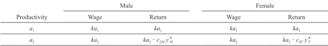
In this equilibrium, wage is effectively determined to be proportional to productivity and equates with that in the complete information condition. Table 1 shows the equilibrium wage and return as a function of productivity and gender.7)
4. 2
Gender Gaps in the Separating Equilibrium
I will show that, in the separating equilibrium, the gender gap in education appears but that in wage does not. Although I still utilize a one employer and one employee model, the assumptions of Bertrand competition and homogeneity of members of the same category may enable us to generalize its results to plural employer and/or plural employee situations, as I suggested in Section 3.1.
Let us assume a uniform distribution for y*M and y*F respectively, because the employer
seems indifferent to the values of them in so far as they fall within the above-mentioned intervals and the potential employeeʼs best response is to choose the level of education that the employer would designate as the critical value in the wage schedule.
Proposition 1. (Gender Gap in Education)
The mean educational level for men is greater than that for women. Proof.
Assuming a uniform distribution for y*M and y*F respectively, we get
E ( y*M) =k ( c1M+c2M) ( a2-a1)
2c1M c2M
and
Table 1 Wage and Return in the Separating Equilibrium
Male Female
Productivity Wage Return Wage Return
a1 ka1 ka1 ka1 ka1
a2 ka2 ka2-c2M yM* ka2 ka2-c2F y*F
Notes: a2> a1 ; c2G is the slope of the educational cost function for an employee of higher productivity; y*G is the educational level
E ( y*F) =k ( c1F+c2F) ( a2-a1)
2c1F c2F
Taking the difference between the two, we get E ( y*M)-E ( y*F) =k ( a2-a1) 2 ⎛⎝cc1M1M+c c2M2M -c1F+c2F c1F c2F ⎞ ⎠ =k ( a2-a1) 2
⎡
⎣
c1M c1F ( c2F −c2M)+c2M c2F ( c1F−c1M) c1M c2M c1F c2F⎤
⎦
Since a2> a1> 0, c1F> c1M> 0, and c2F> c2M> 0, E ( y*M) > E ( y*F).The mean, or the expected value, of educational level for men and that for women are expressed as E ( y│M ) = ( 1-q ) E ( y*M) + q×0 = ( 1-q ) E ( y*M)
and
E ( y│F ) = ( 1-q ) E ( y*F) + q×0 = ( 1-q ) E ( y*F) respectively. Thus, we have
E ( y│M ) > E ( y│F ). □ Proposition 2. (No Gender Gap in Wage)
The mean wage for men is equivalent to that for women. Proof.
The employer will pay ka1 to the employees whose productivity is equal to a1 and ka2 to the
employees whose productivity is equal to a2 (Table 1). The proportion of the former type of
employees is equal to q and that of the latter type is equal to 1-q (Assumption 1). These apply to both men and women. Thus, we have
E ( w│M ) = qka1+ ( 1-q ) ka2
and
E ( w│F ) = qka1+ ( 1-q ) ka2.
E ( w│M ) = E ( w│F ). □
Contrary to Aigner and Cainʼs (1977) conjecture, there would be no gender gap in wage in the separating equilibrium of our generalized version of Spenceʼs (1974a) signaling game with an index, although the assumption of the gender difference in educational cost certainly leads to the prediction of the gender gap in educational attainment.
4. 3
Gender Gaps in the Other Classes of Equilibria
As I noted earlier, we may have other classes of Perfect Bayesian Equilibria: pooling equilibria, hybrid equilibria, and composite equilibria. Although they cannot survive the Intuitive Criterion, these classes of equilibria might be successful in predicting not only the gender gap in education but also that in wage. Thus, I will examine the predicted gender gaps in these classes of equilibria as well.
4. 3. 1
Pooling Equilibria
In our example, the condition that the potential employee chooses y = 0 regardless of his or her productivity and gender constitutes a pooling equilibrium. The potential employeeʼs choice is the best response to the wage schedule in which the employer chooses ycM≥ k ( a2-a1) ⁄ c2M for men
and ycF≥ k ( a2-a1) ⁄ c2F for women. We can find another pooling equilibrium in which the potential
employee chooses y+
G = ycG such that 0 < ycG< k ( a2-a1) ⁄ c1G ( G = M, F ) as his or her educational
level regardless of his or her productivity.
In either case, the employer cannot update his or her initial belief so that he or she has to keep relying on the prior distribution. Since the employer cannot tell whether the potential employeeʼs productivity is higher or lower, the former will pay k [ qa1+ ( 1-q ) a2] to the latter
regardless of productivity and gender (Gibbons 1992, p.196).
On the one hand, in the pooling equilibrium y+= 0, we predict no gender gaps, whether in
education or in wage, that is, E ( y│M ) = E ( y│F ) and E (w│M ) = E (w│F ). The equilibria cannot explain the actual gaps in either case.
On the other hand, in the pooling equilibrium y+
G = ycG ( 0 < ycG< k ( a2-a1) ⁄ c1G), if we
assume a uniform distribution for y+
M and y+F respectively, we can show that E ( y│M ) > E ( y│F )
but E (w│M ) = E (w│F ).
4. 3. 2
Hybrid Equilibrium
In a hybrid equilibrium, at least one type of the potential employee chooses a mixed strategy (Gibbons 1992:186; Fudenberg and Tirole 1991:327). There may be enormous numbers of hybrid equilibria of a signaling game in general. Among these, students of educational signaling in labor markets consider the following case the most important: one type of employee chooses a level of education with certainty while the other type randomizes between the same level of education as the former type and a different level from the former type (Gibbons 1992:202-205; Sawaki 2014:57-61). More specifically, the low productivity type might try to masquerade by having recourse to a mixed strategy when the high productivity employee always chose an educational level that separates him- or herself from the low productivity employee.
into adaptive dynamics, and found that pooling and hybrid equilibria may be likely in replicator and best response dynamics. He argued that a greater appreciation of the hybrid equilibria might promote our understanding of the plausible situations in which low productivity job applicants would masquerade as high productivity ones by investing in the same level of education as the high productivity ones do.
If the high productivity employee played a separating equilibrium strategy, the low productivity employeeʼs motivation to adopt a hybrid equilibrium strategy instead of the separating equilibrium strategy could be interpreted as masquerading. As far as our generalized version of Spenceʼs (1974) signaling game with an index concerns, however, there is no hybrid equilibrium in which the low productivity employee tries to be disguised as the high productivity employee who tries to notify the employer of his or her productivity by signaling.
Proposition 3. (No Hybrid Equilibrium in the Interval that Assures Successful Screening) There exists no hybrid equilibrium that satisfies the following conditions:
(1) the employer offers a wage schedule in which the critical value is equal to yhG such that
k ( a2-a1) ⁄ c1G ≤ yhG< k ( a2-a1) ⁄ c2G ( G = M, F ),
(2) the high productivity employee plays a pure strategy yhG, which could be a separating
equilibrium strategy, and
(3) the low productivity employee plays a mixed strategy assigning the probability p to yhG and
1-p to 0 where 0 < p < 1. Proof.
See Appendix. □
In the same way, we can show that there exists a hybrid equilibrium in which (1) the employer offers a wage schedule whose critical value is equal to y+
G such that 0 < y+G< k ( a2-
a1) ⁄ c1G, (2) the high productivity employee plays a pure strategy y+G, and (3) the low productivity
employee plays a mixed strategy whose support consists of y+
G and 0, if and only if ( 1-q ) ( 1
-qh) k ( a2-a1) ⁄ c1G< y+G< ( 1-qh) k ( a2-a1) ⁄ c1G where qh = pq ⁄ [ pq + ( 1-q )] . The low productivity employeeʼs mixed strategy in this case, however, should not be interpreted as masquerading but as cost saving. The only pure strategy equilibrium in this interval
⎛ ⎝( 1-q ) ( 1-cq1Gh) k ( a2-a1), ( 1-qh) k ( a2-a1) c1G ⎞ ⎠
is the pooling equilibrium in which both the high and low productivity employees choose y+ G.
By adopting the hybrid equilibrium strategy instead of the pooling equilibrium strategy, the low productivity employee not only pays less cost but also reduces the probability that the employer believes he or she is the high productivity employee, although the probability remains positive.
In the hybrid equilibrium, we find a gender gap in education but none in wage, that is, E ( y│M ) > E ( y│F ) and E ( w│M ) = E ( w│F ).8)
4. 3. 3
Composite Equilibrium
Since we introduce gender as an index to the signaling game, we need to consider another class of equilibria that may be called composite equilibria, as well. In a composite equilibrium, a separating equilibrium holds for one gender group and a pooling equilibrium for the other. For our purpose of explaining the gender gaps in education and wage, the most significant is the case in which a male employee plays the separating equilibrium strategy while a female employee plays the pooling equilibrium strategy. On the one hand, a male employee will choose y*M as his educational level if
his productivity is equal to a2 while he will choose y = 0 if his productivity is equal to a1. On the
other hand, a female employee will choose y = 0 regardless of her productivity9) (see Model 3b in
Spence (1974a:Chapter 5) for a numerical example).
In the composite equilibrium, E ( y│M ) > E ( y│F ) and E ( w│M ) = E ( w│F ). Moreover, examination of the gender gap in conditional wage reveals that E ( w│0, M ) < E ( w│0, F ) since ka1-k [ qa1+ ( 1-q ) a2] = k ( 1-q ) ( a1-a2) < 0. In other words, in the composite equilibrium,
among those who did not attain higher education, men would earn less than women on average. This is contrary to what we observe in reality (remember Figure 2).
4. 4
Summary of the Gander Gaps in Various Classes of Equilibria
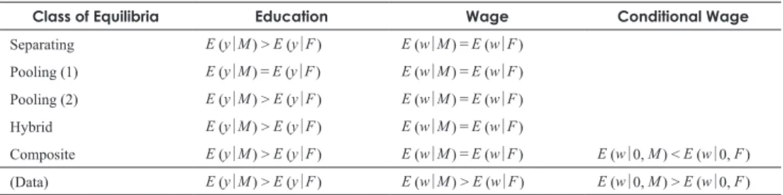
Results are summarized in Table 2. Although this table may not encompass all the possible equilibria, it covers major ones that previous studies examined. On the one hand, the four classes of equilibria, except the pooling equilibrium in which the potential employee choose y = 0 regardless of productivity and gender, the gender gap in education is predicted. On the other hand, no classes of equilibria succeed in predicting the gender gap in wage. Furthermore, in the composite equilibrium where a male employee plays the separating equilibrium strategy but a female employee plays the pooling equilibrium strategy, among those who did not attain higher education, men would earn less than women on average.
Table 2 Predicted Gender Gaps in Education and Wage in Various Equilibria
Class of Equilibria Education Wage Conditional Wage
Separating E (y│M) > E (y│F) E (w│M)=E (w│F)
Pooling (1) E (y│M)=E (y│F) E (w│M)=E (w│F)
Pooling (2) E (y│M) > E (y│F) E (w│M)=E (w│F)
Hybrid E (y│M) > E (y│F) E (w│M)=E (w│F)
Composite E (y│M) > E (y│F) E (w│M)=E (w│F) E (w│0, M) < E (w│0, F) (Data) E (y│M) > E (y│F) E (w│M) > E (w│F) E (w│0, M) > E (w│0, F) Notes: Pooling (1) refers to the pooling equilibrium in which the educational level is equal to 0, while Pooling (2) refers to the equilibrium in which the educational level is greater than 0. In the hybrid equilibrium, the high productivity employee chooses y+
G while the low productivity employee adopts a mixed strategy whose support consists of y+G and 0. The composite equilibrium
consists of a separating equilibrium for a male employee and a pooling equilibrium y+
5
Discussions
Our model succeeded in predicting the gender gap in education but did not in predicting the gender gap in wage. The result suggests that, for the development of a more appropriate model of statistical discrimination in hiring, we need a new approach to belief formation that enables us to explain how the posterior distribution of productivity is differentiated with respect to gender.
5. 1
Employer s Belief Reconsidered
Why does the model fail to predict the gender gap in wage? The reason is as follows. In the separating equilibrium, as the employer is assumed to know that the educational cost for women is greater than that for men, he or she would believe that women with a lower level of education y*F
have the same productivity as men with a higher level of education y*M and therefore offer the same
amount of wage for the women as for the men. This is a logical consequence of the application of Bayesʼ rule to the employerʼs belief updating. Similarly, in other equilibria, the employer would believe that some of women with a lower level of higher education or even with no higher education belong to the type a2, that is, the higher productivity type.
If we regard the reasoning as rational (or reasonable) but the consequence as odd, we may need to propose an alternative approach to belief formation. A “cognitive rationality” approach (e.g. Boudon 1996; see also Oppʼs [2014] criticism) is one of the candidates.
5. 2
Gender-Differentiated Distribution of Productivity?
Although I adopted here an identical prior distribution of productivity for men and women, Arai (1998) assumes a group-differentiated prior distribution of productivity in explaining the concept of statistical discrimination. The difference of the two approaches may correspond to Tomaskovic-Levey and Skaggsʼs (1999, p.424) distinction between two versions of statistical discrimination theory, that is, the strong one and the weak one. They argue that the former, typically adopted by economists such as Aigner and Cain (1977) and Haagsma (1993), assumes the actual existence of the average group differences in productivity, while the latter, typically proposed by sociologists such as Bielby and Baron (1986) and England (1992), emphasizes biased beliefs and stereotypes about productivity rather than actual productivity.10)
The assumption of a gender-differentiated prior distribution of productivity might enable us to prove the existence of the gender gap in wage. Explanation in terms of the theory of statistical discrimination, however, will be convincing when the posterior distribution of productivity is differentiated with respect to gender despite the identical prior distribution, as Anderson, Fryer and Holt (2006, p.105) suggested in praising Arrowʼs (1973) model.
Santos-Pintoʼs (2012) signaling model might seem to have succeeded in convincingly explaining the gender wage gap while assuming an identical prior distribution of productivity for men and women. He claims that even if men and women have the same prior distribution of productivity the gender difference in self-confidence can lead to the gender wage gap. He concludes from the analysis of his model that the mean wage of male employees will be higher than that of female employees if some men are overconfident, some women are underconfident, and education increases productivity. To the result, however, an additional assumption that education raises productivity is critical. In this sense his model is a hybrid of human capital and signaling
approaches rather than a genuine signaling game. As he himself admits, if education does not have an influence on productivity, the model predicts that there is no gender wage gap.
The above discussions suggest that it will be a tough task to construct a good model of statistical discrimination. We should try to do it nevertheless, if we would like to explain the gender gap in wage.
6
Concluding Remarks
Adherents of Spenceʼs (1974a) model of educational signaling in labor markets might assert that its merit lies in addressing the problem of efficiency of educational system and/or statistical discrimination. Nevertheless, before the examination of the problem, we should check whether the model can explain the disparities that we observe. This paper showed how it fails.
It would be precipitate, however, to throw away the concepts of statistical discrimination and/or information transfer in hiring processes. We should quest for a better model with retaining these concepts instead.
Appendix. Proof of Proposition 3
For convenience, we may drop the suffix for gender. Suppose that there existed a hybrid equilibrium in which the employer offered a wage schedule with the critical value of k ( a2-a1) ⁄ ( c1≤ yc< k ( a2
-a1) ⁄ c2), the high productivity employee would always choose yh = yc, and the low productivity employee would choose yh = yc with the probability p and 0 with the probability 1-p ( 0 < p < 1 ).
Applying Bayesʼ rule after observing yh and 0, the employer should believe that
P ( a1│yh) =pq + ( 1pq-q ) P ( a2│yh) = 1 −q pq + ( 1-q ) P ( a1│0 ) = 1 and P ( a2│0 ) = 0
(Gibbons 1992, p.202). In the following, we use the notation that qh =pq + ( 1pq-q )
and
1−qh = 1−q pq + ( 1-q )
The wage schedule should be expressed as
⎰( 1-qh) ka2+ qhka1, y ≥ yh w ( y ) =
⎱ka1, 0 ≤ y < yh
The high productivity employee would choose yh if and only if
( 1-qh) ka2+ qh ka1-c2 yh> ka1 or
yh<( 1
-qh) k ( a2-a1) c2
The expected wage for the low productivity employee playing the above mentioned mixed strategy would be equal to
p [ P ( a2│yh) ka2+ P ( a1│yh) ka1] + ( 1-p ) [ P ( a2│0 ) ka2+ P ( a1│0 ) ka1]
= p ( 1-qh) ka2+ [ 1-p ( 1-qh)] ka1. And the expected cost for the employee would be equal to
pc1 yh+ ( 1-p ) 0 = pc1 yh.
Thus, the expected return would be expressed as
p ( 1-qh) ka2+ [ 1-p ( 1-qh)] ka1-pc1 yh.
The low productivity employee would be motivated to play the mixed strategy if and only if p ( 1-qh) ka2+ [ 1-p ( 1-qh)] ka1-pc1 yh> ka1.
(Otherwise, he or she could maximize his or her utility by always choosing y = 0, which would yield a separating equilibrium.) Rearranging this inequality, we get the condition that
yh<( 1
-qh) k ( a2-a1) c1
Since ( 1-qh) k ( a2-a1) ⁄ c1< k ( a2-a1) ⁄ c1 this condition contradicts the assumption that k ( a2-a1) ⁄ c1≤ yh< k ( a2-a1) ⁄ c2. □
Acknowledgements
Part of this study was supported by Japan Society for the Promotion of Science Grants-in-Aid for Challenging Research (Exploratory), Number JP17K18571, “Mathematical Models of Stigma and
Passing.” The core idea and numerical examples were presented at Advances in Rational Choice Social Research, Preconference of the Rationality and Society Section, 108th Annual Meeting of the American Sociological Association, New York, USA, 9 August 2013 (“Can the Signaling Game Serve as a Model of Statistical Discrimination?”). An earlier version of this paper (“Signals, Indices, and Statistical Discrimination in Hiring”) was presented at the session on Rational Choice and Inequalities in the Life Course, RC45 (Rational Choice), the 3rd Forum of Sociology, Vienna, Austria, 11 July 2016. I appreciate comments from Antonio Chiesi, Michio Umino, and the two anonymous reviewers.
Notes
1) The indicator is defined as 100×(1-Mf ⁄ Mm)(%), where Mf stands for median earnings of female full-time
employees and self-employed workers, and Mm stands for those of male counterparts.
2) Figure 2 only serves as a rough estimation of the gender gap. The starting salary varies depending on occupation, firm size, industrial sector, and other relevant factors.
3) Arai (1995:62-65) and Spence (1974a:38-46) differ in the reference of the indices. Spence assumed race, while Arai assumed descent or family origin that determines parentsʼ wealth in the analysis of a formal model and gender in unmathematical discussion. They also differ in the assumption of the distribution of employeesʼ productivity.
4) Another problem of Cho and Krepsʼs (1987) assumption is that it obscures the difference between signaling theory and human capital (Becker [1964] 1993) theory.
5) If the employer finds that education is not efficient in screening, however, he or she will pay on the basis of an expected productivity of the potential employee.
6) The employer may instead modulate the critical value in the wage schedule in order that it should satisfy the inequality k (a2-a1) ⁄ c1G≤ ycG< k (a2-a1) ⁄ c2G. However, this is rather a problem of equilibrium selection.
7) The condition that y*G = ycG< k (a2-a1) ⁄ c2G (G = M, F) implies that the low productivity employee could be
said to envy the return that the high productivity employee attains when the screening is successful, that is,
w (0│a1)-c (0│a1) < w (yG*│a2)-c (y*G│a2) (Gibbons 1992:194).
8) In the hybrid equilibrium, we have E (y│G) = (1-q) y+
G+ q [ py+G+ (1-p)0 ] = [ pq + (1-q)] y+G and (1-q)
(1-qh) k (a2-a1) ⁄ (c1G<y+G< (1-qh) k (a2-a1) ⁄ c1G) (G = M, F) where qh = pq ⁄ [ pq + (1-q)] . Assuming a
uniform distribution for y+
M and y+F respectively, we get E (y│M) > E (y│F) since c1F> c1M. The expected wage
for a low productivity employee is equal to p (1-qh) ka2+ [1-p (1-qh)]ka1 where 0 < p < 1, and that for a
high productivity employee is equal to (1-qh) ka2+ qh ka1 regardless of gender. As we postulated an identical distribution of productivity for men and women, E (w│M) = E (w│F).
9) If a female employee chooses a pooling equilibrium strategy y = y+
F< k (a2-a1) ⁄ c1F regardless of her
productivity, the resulting wage will be the same as that in the case where she chooses y = 0.
10) Note that the standard formulations of a signaling game as an incomplete information game, including a generalized version of Spenceʼs (1974a) signaling model in this paper, implicitly or explicitly assume that the actual distribution of productivity is common knowledge and therefore adopt it as the prior distribution (e.g. Cho and Kreps 1987:187; Gibbons 1992:202; Sawaki 2014:4).
References
Aigner, Dennis J., and Glen G. Cain, 1977, “Statistical Theories of Discrimination in Labor Markets,” Industrial and
Labor Relations Review, 30(2):175-187.
Anderson, Donna M., and Michael J. Haupert, 1999, “Employment and Statistical Discrimination: A Hands-On Experiment,” Journal of Economics (The Missouri Valley Economic Association), 25(1):85-102.
Anderson, Lisa R., Roland G. Fryer, and Charles A. Holt, 2006, “Discrimination: Experimental Evidence from Psychology and Economics,” pp.97-115 in Handbook of the Economics of Discrimination, edited by William M. Rodgers III, Edward Elgar.
Arai, Kazuhiro, 1998, The Economics of Education: An Analysis of College-going Behavior, Springer.
Arrow, Kenneth, 1973, “The Theory of Discrimination,” pp.3-33 in Discrimination in Labor Markets, edited by Orley Ashenfelter and Albert Rees, Princeton University Press.
Becker, Gary S., 1957, The Economics of Discrimination, University of Chicago Press.
Becker, Gary S., [1964] 1993, Human Capital: A Theoretical and Empirical Analysis with Special Reference to
Education, 3rd ed., University of Chicago Press.
Bertrand, J., 1883, «Théorie des richesses. Théorie mathématique de la richesse sociale, par Léon Walras, professeur dʼéconomie politique à lʼacademie Lausanne, Lausanne 1883. Recherches sur les principes mathématique de la
théorie de richesses, par Augustin Cournot, Paris 1838,» Le Journal des sçavans (Septembre 1883), pp.499-508.
Bielby, William T., and James N. Baron, 1986, “Men and Women at Work: Sex Segregation and Statistical Discrimination,” American Journal of Sociology, 91(4):759-99.
Blume, Lawrence E., 2006, “The Dynamics of Statistical Discrimination,” Economic Journal, 116(515):F480-F498. Boudon, Raymond, 1996, “The ʻCognitivist Modelʼ: A Generalized ʻRational Choice Modelʼ,” Rationality and Society,
8(2):123-50.
Cho, In-Koo, and David M. Kreps, 1987, “Signaling Game and Stable Equilibria,” Quarterly Journal of Economics, 102(2):179-222.
Coate, Stephen, and Glenn Loury, 1993, “Will Affirmative Action Eliminate Negative Stereotypes?” American
Economic Review, 83(5):1220-40.
England, Paula, 1992, Comparable Worth: Theory and Evidence, Aldine de Gruyter.
Ewens, Michael, Bryan Tomlin, and Liang Choon Wang, 2014, “Statistical Discrimination or Prejudice? A Large Sample Field Experiment,” Review of Economics and Statistics. 96(1):119-134
Fang, Hamming, and Andrea Moro, 2011, “Theories of Statistical Discrimination and Affirmative Action,” pp.133-200 in Handbook of Social Economics, Vol.1A, edited by Jess Benhabib, Matthew O. Jackson, and Alberto Bisin, North-Holland.
Fryer, Roland G., Jr., 2007, “Belief Flipping in a Dynamic Model of Statistical Discrimination,” Journal of Public
Economics, 91(5-6):1151-66.
Fudenberg, Drew, and Jean Tirole, 1991, Game Theory, MIT Press. Gibbons, Robert, 1992, A Primer in Game Theory, Harvester Wheatsheaf.
Haagsma, Rein, 1991, “Statistical Discrimination and Competitive Signalling,” Economics Letters, 36:93-7.
Moro, Andrea, and Peter Norman, 2004, “A General Equilibrium Model of Statistical Discrimination,” Journal of
Economic Theory, 114(1):1-30.
OECD, 2016, Education at a Glance 2016.
OECD, 2019, “Gender wage gap (indicator),” doi:10.1787/7cee77aa-en, accessed on 14 February 2019 (https://data. oecd.org/earnwage/gender-wage-gap.htm).
Opp, Karl-Dieter, 2014, “The Explanation of Everything: A Critical Assessment of Raymond Boudonʼs Theory Explaining Descriptive and Normative Beliefs, Attitudes, Preferences, and Behavior,” Revista de Sociologia, 99(4):481-514.
Phelps, Edmund S., 1972, “The Statistical Theory of Racism and Sexism,” American Economic Review, 62(4):659-61. Santos-Pinto, Luís, 2012, “Labor Market Signaling and Self-Confidence: Wage Compression and the Gender Pay
Gap,” Journal of Labor Economics, 30(4):873-913.
Sawaki, Hisashi, 2014, The Game Theory of Signaling (in Japanese), Keiso Shobo.
Schwab, Stewart, 1986, “Is Statistical Discrimination Efficient?” American Economic Review, 76(1):228-34. Spence, A. Michael, 1974a, Market Signaling: Informational Transfer in Hiring and Related Screening Processes,
Harvard University Press.
Spence, A. Michael, 1974b, “Competitive and Optimal Response to Signals: An Analysis of Efficacy and Distribution,” Journal of Economic Theory, 7:296-332.
Statistics Bureau, Ministry of Internal Affairs and Communications, Japan, (n.d.), “e-Stat: Portal Site of Official Statistics of Japan,” (Retrieved February 14, 2019, https://www.e-stat.go.jp/).
Tomaskovic-Devey, Donald, and Sheryl Skaggs, 1999, “An Establishment-Level Test of the Statistical Discrimination Hypothesis,” Work and Occupations, 26(4):422-45.
Vincent-Lancrin, Stéphan, 2008, “The Reversal of Gender Inequalities in Higher Education: An On-going Trend,” pp.265-298 in Higher Education to 2030, Volume 1, Demography, OECD.
Wagner, Elliot O., 2013, “The Dynamics of Costly Signaling,” Games, 4:163-81.
木村 邦博(きむら くにひろ).東北大学大学院文学研究科 教授.〒 980-8576 宮城県仙台市青葉区川内 27-1. kkimura@tohoku.ac.jp.研究関心:数理計量社会学,合理的選択理論,社会調査法.