Steady State Analysis of the TCP Network with RED Algorithm

全文

(1)IEICE TRANS. FUNDAMENTALS, VOL.E99–A, NO.6 JUNE 2016. 1247. LETTER. Steady State Analysis of the TCP Network with RED Algorithm Daisuke ITO†a) and Tetsushi UETA†† , Members. SUMMARY The transmission control protocol with a random early detection (TCP/RED) is an important algorithm for a TCP congestion control [1]. It has been expressed as a simple second-order discrete-time hybrid dynamical model, and shows unique and typical nonlinear phenomena, e.g., bifurcation phenomena or chaotic attractors [2], [3]. However, detailed behavior is unclear due to discontinuity that describes the switching of transmission phases in TCP/RED, but we have proposed its analysis method in previous study. This letter clarifies bifurcation structures with it. key words: TCP/RED, S-model, border-collision bifurcation. 1.. Introduction. With the progress of computer technology, packet routing methods have become serious problems. Especially, a network congestion avoidance technology is one of the critical issues [4], [5]. If many senders transmit a lot of packets to a network at the same time, tandem switches and receivers will overflow with them, disorderly transmissions of senders will decrease throughputs of local or global computer networks drastically. Thus, appropriate protocols that guarantee the throughput are necessary, and the congestion avoidance technology that routers monitor and adjust the flow of a network has been proposed [6]. In 1988, the TCP Tahoe was proposed as the congestion avoidance with a slow-start algorithm [7]. This is a simple window-based process: at first, the sender sets the window size as a narrow value since it has no information about a network condition. After that, the upload bandwidth (the window size) is expanded gradually. If the congestion occurs by an excessive expansion of window sizes and a lot of packets, senders will reset the window size as the slow-start phase. Hence, the increase of packets can be suppressed. The TCP Reno, which has a fast recovery algorithm, was introduced in the early 1990 [8]. When a packet drop occurs, the TCP Tahoe has tendency decreased the window size too small. The TCP Reno has alleviated this problem by the fast recovery phase. These techniques are based on the window-based congestion controlling method [7]. On the other hand, the Random Early Detection (RED), is an Active Queue Management (AQM) scheme, was proposed in 1993 by Floyd [1], [9]. This method is employed along with the TCP congestion control mechanisms in order Manuscript received January 7, 2016. Manuscript revised February 17, 2016. † The author is with The University of Shiga Prefecture, Hikone-shi, 522-8533 Japan. †† The author is with Tokushima University, Tokushima-shi, 770-8506 Japan. a) E-mail: [email protected] DOI: 10.1587/transfun.E99.A.1247. to increase further the throughput of the computer network. It is conceivable that this method improves the performance of network and fairness to senders [10]. Thus, it is the important algorithm for the congestion avoidance. In recent year, there have been many investigations of TCP/RED with numerical simulations [2], [11]. Mathematical models of these techniques are studied actively to investigate reliance with parameters [12]. The S-model, proposed by Zhang et al., has good approximation of TCP/RED without random numbers, and it is used for numerical simulations [2]. It is described as a discrete-time hybrid dynamical system, and occurs global bifurcation phenomena; border-collision (BC) bifurcation phenomena are reported in Ref. [3]. However, most of previous studies are focused on the performance with varying parameters and the its design because the configuration of TCP/RED parameters requires an empirical knowledge. On the other hand, the investigation of these bifurcation structures helps an understanding of global behavior. The analysis of bifurcation structures of the model is seldom studied, because we had no way to determine parameter sets of bifurcation phenomena for hybrid dynamical systems due to non-smoothness on the state space. Hence, the detailed investigation of bifurcation structures of the S-model was not enough. In our previous study, we have proposed the analysis method based on the Newton’s method for determination of bifurcation parameters of hybrid dynamical systems [13]. It is accomplished owing to an extent border line defined by threshold values, and can analyze approximately detailed bifurcation structures of border collision bifurcations for hybrid dynamical systems. In this letter, we try to clarify the bifurcation structure of the S-model in detail. At first, we explain the analysis method for them, after that we show some bifurcation structures, and demonstrate behavior of the model with varying parameters. 2. S-Model Constructed from TCP/RED First of all, let us explain the S-model constructed from TCP/RED [2]. Assume that pk is the drop probability of a packet, Wk and qk mean the window size and the average queue size, respectively, and they are state variables of the model q = (W, q)⊤ . The S-model is shown below. • The drop probability of a packet pk. c 2016 The Institute of Electronics, Information and Communication Engineers Copyright ⃝.

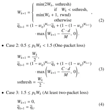
(2) IEICE TRANS. FUNDAMENTALS, VOL.E99–A, NO.6 JUNE 2016. 1248 Table 1 Parameters of the TCP network. Receiver advertised window size (rwnd[packets]) 1, 000 Link capacity (C[bps]) 1.54 × 106 Round-trip propagation delay (d[sec]) 22.8 × 10−3 Packet size (M[bits]) 4, 000. Fig. 1 Structure of the drop probability of a packet. When q is less than qmin , p is set for zero, thus all packets will be received without loss of packets.. pk+1.  0       1 =  qk+1 − qmin    pmax  qmax − qmin. if qk+1 ≤ qmin if qk+1 ≥ qmax otherwise (1). where, qmin and qmax are the minimum and maximum queue threshold values, respectively. pmax is the maximum packet drop probability. They determine the value of pk . Figure 1 sketches the shape of Eq. (1). • Case 1: pk Wk < 0.5 (No loss)  min(2Wk , ssthresh)      if Wk < ssthresh,  , Wk+1 =   min(W + 1, rwnd)  k    otherwise (2) qk+1 = (1 − wq )W(k+1 qk + (1 − (1 −)wq )Wk+1 ) C·d · max Wk+1 − ,0 . M • Case 2: 0.5 ≤ pk Wk < 1.5 (One-packet loss) Wk , 2 qk+1 = (1 − wq )W(k+1 qk + (1 − (1 −)wq )Wk+1 ) C·d · max Wk+1 − ,0 , M Wk ssthresh = . 2 Wk+1 =. (3). • Case 3: 1.5 ≤ pk Wk (At least two-packet loss) Wk+1 = 0, qk+1 = qk .. (4). ssthresh means the threshold value of a congestion window size, and rwnd, C, d, and M are parameters of the TCP network, and we employ these parameters as Table 1 [2]. wq is the weight factor of a low-pass filter to get the average queue size qk . Especially, qmax , qmin , pmax and wq are adjustable parameters of TCP/RED, and others are constant parameters. The S-model can be considered as a two-dimensional hybrid dynamical system, and it is composed of 11-tuple maps from Eqs. (1)–(4). Subspaces for each map are shown in. Fig. 2 Subspace for 11-tuple maps. This figure indicates seven subspaces only. The others are located in outside of this range, or they have no areas, e.g. generally rwnd is set as large value, and Wk is always smaller than it.. Fig. 2. Note that, subspaces are illustrated only seven areas because some maps have no regions in which the conditions of some maps are satisfied on the state space with normal settings of parameter values. 3. Bifurcation Analysis It is generally difficult to determine bifurcation parameters in hybrid dynamical systems by discontinuity of a state space, e.g., a hysteresis or a switch [14]. Discrete time hybrid dynamical systems are described as piecewise smooth functions, and they have an interrupt characteristic. It causes some problems for the analysis of bifurcation structures, but in our previous study analysis method for discrete time hybrid dynamical systems has been proposed [13]. The hybrid system is defined as follows: xk+1 = f (xk ) = fi (xk ) if. xk ∈ Di ,. (5). where xk ∈ Rn is the state, f is a function satisfying f : Rn 7→ Rn . fi , i = 1, 2, . . . m are C ∞ -class functions that are used on subspace Di . Thus, the applied functions are selected from fi , depending on the location of the current state xk . The solution φ is defined as xk = φ(x0 , k),. (6). where x0 is the initial value, which satisfies x0 = φ(x0 , 0). The detection of bifurcation parameters is difficult because Eq. (6) has non-smoothness on boundaries between two subspaces. If periodic points that satisfy Eq. (7) exist, the Jacobian matrix of a discrete time system is expressed as: x∗0 = φ(x∗0 , p).. (7).

(3) LETTER. 1249. ∂φ ∂ f ∂φ ∂φ (k + 1) = (k), (0) = I, ∂x0 ∂x ∂x0 ∂x0. (8). where ∂φ/∂x0 (k) represents the Jacobian matrix, which can estimate the stability of periodic points. However, in the case of a hybrid dynamical system, f is a C 0 -class function. To analyze the stability of the solution and to detect its bifurcation parameters, the Jacobian matrix is necessary, but it accomplished by using derivative of Eq. (6). In hybrid dynamical systems, function f is selected from fi , according to the state x. Additionally, the derivation of maps can be expressed by the same way. The Jacobian matrix is also calculated as follows:

(4) ∂φ ∂φ ∂ fi

(5)

(6) ∂φ

(7)

(8) (k + 1) = (k), (0) = I. (9) ∂x0 ∂x x ∈D ∂x0 ∂x0 k. i. The shooting method can be applied to solve Eq. (7) by using these equations. The border-collision bifurcation is the characteristic phenomena in the hybrid dynamical system, and it occurs when periodic points across the border that defines each subspace. It can be analyzed by adding the function defines the border to the recurrence formula of the shooting method, and they are expressed as follows: F(λ) = η(φ(λ)) = 0 ∂η(λ) ∂φ F ′ (λ) = =0 ∂q ∂λ. Fig. 3 Bifurcation diagram in the pmax –wq plane. other parameters are qmin = 5, qmax = 15, ssthresh = 20, and Table 1. All of bifurcation phenomena in this parameter ranges are BC-bifurcations.. (10) (11). where λ is the parameter, e.g., wq , pmax and so on. The Jacobian matrix is computed by Eq. (8). Note that, ∂φ/∂λ is given by

(9)

(10) ∂φ ∂ fi

(11)

(12) ∂ fi

(13)

(14) ∂φ

(15)

(16) (k + 1) = (k) + (12) , ∂λ ∂x

(17) xk ∈Di ∂x0 ∂λ

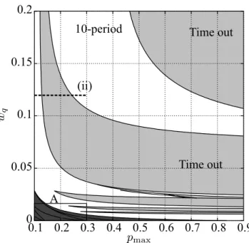
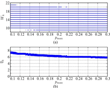
(18) xk ∈Di ∂φ (13) (0) = 0. ∂λ Additionally, in analysis of the border collision bifurcation, there is the serious problem explained, but we proposed the its workaround technique [13]. In this letter we use above shooting method and expansion borders for the BC bifurcation analysis. 4.. Analysis Results. We analyze bifurcation structures of the S-model. Figure 3 shows the two-parameter bifurcation diagram in the pmax – wq plane. The system with parameters on gray regions occurs the “At least two-packet loss”. The time out occurs because of dropping some consecutive packets; hence senders close the window size and have to wait the idle time. As a result, the throughput of the router will decrease. All bifurcation phenomena in this parameter ranges are bordercollision (BC) bifurcations, and some bifurcation sets have Arnold tongue structures. Figure 4 shows the magnification diagram of Fig. 3. It is confirmed that various periodic regions exist and they have an Arnold tongue structure. These. Fig. 4 Magnified figure of rectangle A in Fig. 3. Various periodic attractors are embedded in this region. The numbers in the figure show the periods of attractors.. parameter sets are also BC bifurcations. The one-dimensional bifurcation diagram varied the parameter pmax on the line (i) (wq = 0.002) in Fig. 4 is shown in Fig. 5. Figures 5(a) and (b) shows Wk and qk respectively. Many BC bifurcations happen, and they cascade with varied pmax . The average queue size decreases slowly. Therefore, the BC bifurcation phenomena affect the performance of TCP/RED. Figure 6 shows one-dimensional bifurcation diagram with wq = 0.13 on the line (ii). When wq is increased, Wk and qk has constant values against varying wq ..

(19) IEICE TRANS. FUNDAMENTALS, VOL.E99–A, NO.6 JUNE 2016. 1250. tion structures of the S-model constructed from TCP/RED. From analysis results observed bifurcation phenomena in this mathematical model are mainly BC-bifurcations. From bifurcation diagram Fig. 4, they have formed Arnold tongue structures. From bifurcation structures and one-dimension bifurcation diagrams, the tendency of the performance and parameter regions in which the TCP/RED system occurs the time out and the idle time are clarified. As a result, to alleviate the timeout, and to keep the average queue size, the weight factor should be set as lower values, i.e. wq = 0.002, but the timeout caused by dropping multi packets will occur when the max drop probability pmax is set as the large value by BC bifurcations. Acknowledgement Fig. 5 One-dimensional bifurcation diagram varied the parameter pmax on the line (i) in Fig. 4. (wq = 0.002) (y-axis: the window size Wk and the average queue size qk [packets]).. This work has been supported by JSPS KAKENHI Grant Number 25420373. References. Fig. 6 One-dimensional bifurcation diagram varied the parameter pmax on the line (ii) in Fig. 4. (wq = 0.13) (y-axis: the window size Wk and the average queue size qk [packets]).. On the line (ii), BC bifurcations do not occur with varying wq , and it is easy to see by the comparison with Fig. 4. Therefore steady state of the model is not changed, and state variables have the same vale for various wq . However, the average queue sizes have sparse values than the wq = 0.002 case, and include small values. Thus the throughput of the model is lower than previous one. Moreover, the time out happens at the middle value of pmax (the shaded region). As a result, in the S-mode, it can be considered that the weight wq should be set as lower value, e.g. wq = 0.002, thus weak low-pass filter is suitable for this network [2]. 5.. Conclusion. In this letter, we have investigated the stability and bifurca-. [1] S. Floyd and V. Jacobson, “Random early detection gateways for congestion avoidance,” IEEE/ACM Trans. Netw., vol.1, no.4, pp.397–413, Aug. 1993. [2] H. Zhang, M. Liu, V. Vukadinović, and L. Trajković, “Modeling TCP/RED: A dynamical approach,” Complex Dynamics in Communication Networks, Understanding Complex Systems, pp.251–278, Springer-Verlag Berlin/Heidelberg, 2005. [3] M. Liu, A. Marciello, M. di Bernardo, and L. Trajkovic, “Discontinuity-induced bifurcations in TCP/RED communication algorithms,” Proc. 2006 IEEE International Symposium on Circuits and Systems, ISCAS 2006, 2006. [4] J. Postel, “Transmission control protocol,” Tech. Rep. 793, Request for Comment (RFC), Sept. 1981. [5] M. Allman, V. Paxson, and W. Steven, “TCP congestion control,” Tech. Rep. 2581, Request for Comment (RFC), April 1999. [6] V. Jacobson, “Congestion avoidance and control,” SIGCOMM Comput. Commun. Rev., vol.18, no.4, pp.314–329, Aug. 1988. [7] K. Fall and S. Floyd, “Simulation-based comparisons of Tahoe, Reno and SACK TCP,” SIGCOMM Comput. Commun. Rev., vol.26, no.3, pp.5–21, July 1996. [8] J. Padhye, V. Firoiu, D.F. Towsley, and J.F. Kurose, “Modeling TCP Reno performance: A simple model and its empirical validation,” IEEE/ACM Trans. Netw., vol.8, no.2, pp.133–145, April 2000. [9] P. Kuusela, P. Lassila, J. Virtamo, and P. Key, “Modeling RED with idealized TCP sources,” Proc. IFIP ATM & IP 2001, pp.155–166, June 2001. [10] Y. Zhang and L. Qiu, “Understanding the end-to-end performance impact of RED in a heterogeneous environment,” Tech. Rep., Ithaca, NY, USA, 2000. [11] D. Lin and R. Morris, “Dynamics of random early detection,” SIGCOMM Comput. Commun. Rev., vol.27, no.4, pp.127–137, 1997. [12] H. Ohsaki and M. Murata, “Steady state analysis of the red gateway: Stability, transient behavior, and parameter setting,” IEICE Trans. Commun., vol.E85-B, no.1, pp.107–115, Jan. 2002. [13] D. Ito, T. Ueta, T. Kousaka, and K. Aihara, “Bifurcation analysis of the Nagumo-Sato model and its coupled systems,” Int. J. Bifurcation and Chaos, vol.26, no.3, 1630006 (11 pages), March 2016. [14] K. Kinoshita, T. Ueta, H. Kawakami, J. Imura, and K. Aihara, “Bifurcation phenomena of coupled piecewise affine system with hysteresis properties,” Proc. NOLTA 2011, pp.407–410, Sept. 2011..

(20)