The Dynamics of an Eco-Epidemiological Model with Allee Effect and Harvesting in the Predator

(1)

西南交通大学学报

第 55 卷第 2 期

2020 年 4 月

JOURNAL OF SOUTHWEST JIAOTONG UNIVERSITY

Vol. 55 No. 2

Apr. 2020

ISSN: 0258-2724 DOI：10.35741/issn.0258-2724.55.2.29

Research article Mathematics

T

HE

D

YNAMICS OF AN

E

CO

-E

PIDEMIOLOGICAL

M

ODEL WITH

A

LLEE

E

FFECT AND

H

ARVESTING IN THE

P

REDATOR

具有阿利效应的捕食者生态流行病模型的动力学

Huda Abdul Satar

Department of Mathematics, College of Science, University of Baghdad Baghdad, Iraq, [email protected]

Received: January 10, 2020 ▪ Review: March 12, 2020 ▪ Accepted: April 5, 2020

This article is an open access article distributed under the terms and conditions of the Creative Commons Attribution License (http://creativecommons.org/licenses/by/4.0)

Abstract

The aim of this study was to propose and evaluate an eco-epidemiological model with Allee effect and nonlinear harvesting in predators. It was assumed that there is an SI-type of disease in prey, and only portion of the prey would be attacked by the predator due to the fleeing of the remainder of the prey to a safe area. It was also assumed that the predator consumed the prey according to modified Holling type-II functional response. All possible equilibrium points were determined, and the local and global stabilities were investigated. The possibility of occurrence of local bifurcation was also studied. Numerical simulation was used to further evaluate the global dynamics and the effects of varying parameters on the asymptotic behavior of the system.

Keywords: Prey-Predator, Allee Effect, Harvesting, Disease, Bifurcation

摘要这项研究的目的是提出和评估具有阿利效应和捕食者非线性收获的生态流行病学模型。假定猎物中存在一种 SI 型疾病，并且由于猎物的其余部分逃逸到安全区域，因此捕食者只会攻击一部分猎物。还假设捕食者根据改良的霍林二世型功能反应消耗了猎物。确定所有可能的平衡点，并研究局部和全局稳定性。还研究了发生局部分叉的可能性。数值模拟被用来进一步评估全局动力学以及变化的参数对系统渐近行为的影响。 关键词:捕食者，阿利效应，收获，疾病，分叉

(2)

西南交通大学学报

第 55 卷第 2 期

2020 年 4 月

JOURNAL OF SOUTHWEST JIAOTONG UNIVERSITY

Vol. 55 No. 2

Apr. 2020

I. I

NTRODUCTION

The prey–predator interaction and the evolution of species are central topics of investigation in the study of ecological communities. This interaction almost varies in nature in case of presence of infectious diseasesthat affect some or all of the species. Understanding the dynamics of prey–predator pathogens requires the use of mathematical modeling to formulate the model and then analyze the proposed model where one or more of the main populations become infected to an infection. The term eco-epidemiological model isused to describe models that incorporate diseases in ecological communities [1]. The first eco-epidemiological model including an infectious disease in prey was introduced by Anderson and May [2]. Later, a number of researchers proposed and studied eco-epidemiological models involving numerous biological factors; see, for example [3], [4], [5], [6], [7], [8], [9], [10]. It has been observed that the spread of diseases among a population is a main reason for the species’ extinction.

Although many studies have been conducted in the area of eco-epidemiology, the impact of the Allee effect on eco-epidemiological systems has yet to be sufficiently examined. The Allee effect, which is named after Allee [11], has significantly contributed to the study of population dynamics. In fact, Allee effects can be classified as strong or weak [12], [13]. For the strong Allee effect, there is a threshold population level below which the species faces extinction. By contrast, for weak Allee effects, the growth rate decreases but remains positive at low population densities. The research on eco-epidemiological systems under the influence of Allee effects are relatively rare [14], [15], [16], [17], [18], [19], [20]. Recently, Biswas et al. [19] considered a system of delay differential equations to represent prey–predator eco-epidemic dynamics with a weak Allee effect in the growth of the predator population. They observed that there was a threshold for the Allee parameter, above which the predator population will be eliminated from the system. However, Saifuddin et al. [20] explored an eco-epidemiological model with a weak Allee effect in predator population, and a disease in the prey population. They considered a prey-predator model with type II functional response and

concluded that chaotic dynamics can be controlled by the Allee parameter as well as the competition coefficients.

With these considerations in mind, a prey-predator model with disease in the prey populatin and Allee effects in the predator population was proposed, and thus, modified Holling type II functional response was used for predation, which is more realistic in cases with the existence of a predator consuming two types of prey. It was also assumed that there was a Micheal-Mentence type of harvesting for the predator. This paper is organized in the following manner. Section II deals with model formulation. Section III determines the equilibrium points and describes stability analysis. The bifurcation analysis of the system is investigated in section IV. Section V deals with the numerical simulation of the system, and finally, the discussion and conclusion is addressed in Section VI.

II. M

ODEL

F

ORMULATION

In this section,the mathematical model used in this study is formulated, and the dynamics of the prey-predator system is described in a case with the existence of an infectious disease in the prey population and an Allee effect in the predator population, which was carried out according to the following set of hypotheses.

 The prey species consists of two components known as susceptible prey with a density at time given by and infected prey with a density at time given by . However, the predator consists of one component with a density at time given by .

 The susceptible prey species grows logistically with an intrinsic growth rate and a carrying capacity of . While the infected prey cannot grow, it competes with the other species for food and space with an intraspecific competition rate, . Furthermore, the predator population decays exponentially with a disease death rate, .

 The disease transfers by contact between the susceptible and infected individuals according to the prey’s saturated function with an attack rate of and a half saturated constant of

.

 The predator consumes the available portion of the prey species, which is given by

(3)

, after hiding a portion of the prey due to its relocation to the safe property where the prey protect themselves from predation according to the modified Holling type II, with attack rates of , and conversion rates of , for susceptible prey and infected prey, respectively. However, the parameter is the interference between the infected individual, while represents the half saturation constant. In addition, the predator population decays exponentially in the absence of their food due to a natural death rate of .

 The predator population is assumed to be harvested by external forces according to the Micheal-Mentence type of harvesting function with the effort , two different catchability constants , and are the positive harvesting constants.

 Finally, it is assumed thatthe predator population falls under the effects of Allee effect with an Allee constant of .

According to these hypotheses, the dynamics of the eco-epidemiological system can be described using the following set of nonlinear differential equations.

(1)

with and .

Now in order to study the above system of equations more generally, we drop all the units from it by using the following dimensionless variables and constants.

Accordingly, the following dimensionless system is obtained:

(2)

with , and

. Therefore system (2) has the following domain

Clearly,all the interaction functions in the right hand side are continuous and have continuous partial derivatives, and hence the solution of system (2) exists and is unique. Moreover, the solution of system (2) is proved to be uniformly bounded as shown in the following theorem.

Theorem 1: For anyinitial condition belong to , the solution of the system (2) is uniformly bounded in the region

Here is given in the proof.

Proof. From the first equation we have , then it’s easy to verify that for

we get . Now, let ,

then the derivative of with respect to time can

be written as , here

. Then according to the last differential inequality, it’s easy to verify that for , we obtain . Hence the proof is complete.

Keeping the above in view, system (2) describes the dynamics of eco-epidemiological model consisting to susceptible prey, infected prey and predator involving the effects Allee effect and harvesting according to the Micheal-Mentence type model. It has a unique solution moving in the interior of bounded region belongs to the positive octant . Therefore it is important to investigate the asymptotic behavior of the solution of system (2) and their attracting sets as time increases.

III. E

QUILIBRIUM

P

OINTS AND

T

HEIR

S

TABILITY

A

NALYSIS

In the following the conditions of existence all possible equilibrium points of system (2) are established and then the local stability analysis of each of them is studied. Straightforward computation shows that system (2) has at most the following equilibrium points.

The trivial equilibrium point and the axial equilibrium point always exist.

(4)

The predator free equilibriumpoint that located in the interior of positive quadrant of -plane and denoted by exists uniquely provided that

(3a) where

(3b) The infected prey free equilibriumpoint that located in the interior of positive quadrant of -plane and denoted by exists uniquely provided that

(4a) with one of the following set of conditions

(4b) where

(5a) while is a positive root of the following fourth order equation

(5b) where:

with and .

Finally the coexistence or positive equilibriumpoint that located at the interior of positive octant and denoted by

, where

(6)

where ;

, while

represents the intersection point of the foing two isoclines in the interior of positive quadrant of

plane.

(7a)

(7b)

Here ; .

Obviously, as , the above two isoclines become (7c) and (7d) with ; and

Straightforward computation shows that the two isoclines (7c) and (7d) intersects the axis at a unique positive point denoted by and respectively provided that one set of the following sets of sufficient conditions is satisfied.

(7e)

Accordingly, the two isoclines (7c) and (7d) have a unique intersection point given by

belongs to the interior of positive quadrant of plane provided that the following conditions hold.

(5)

(8b) (8c) The local stability analysis of these equilibrium points is investigated using the linearization technique by computing the Jacobian matrix of the system at each of these points and then computes their eigenvalues. Recall that, an equilibrium point is locally asymptotically stable provided that all the eigenvalues of their Jacobian matrix have negative real parts. Now, the general Jacobian matrix of system (2) around the point

can be written as:

(9) here

with ;

and .

Accordingly, with the help of Eq. (9) at each of the above equilibrium point, the following results can be obtained directly for local stability of system (2).

Straightforward computation shows that the Jacobian matrix of system (2) around the trivial equilibrium point has the following eigenvalues:

(10)

Therefore, the origin is always unstable (saddle point).

The Jacobian matrix evaluated at the axial equilibrium point can be written as

(11a)

Therefore the eigenvalues are given by

(11b)

Hence the axial equilibriumpoint is locally asymptotically stable if the following condition holds

(11c)

Now the Jacobian matrix evaluated at the predator free equilibrium point is given by:

(12a)

with and

. Clearly, the eigenvalues of are given by

(12b)

where and

. Therefore these eigenvalues have negative real parts and hence is locally asymptotically stable if and only if the following condition holds.

(6)

Further, the Jacobian matrix evaluated at the infected prey free equilibrium point is given by:

(14a) where

with , ,

and . Consequently the eigenvalues of are given by

(14b)

where:

Hence all these eigenvalues have negative real parts and hence is locally asymptotically stable if and only if the following condition holds.

(15a) (15b)

(15c) Finally, the Jacobian matrix at the coexistence equilibrium point is given by:

(16a)

where . Hence

the characteristic equation of can be written as:

(16b) where

with

Consequently, the local stability of the coexistence equilibrium point of system (2) can be discussed in the following theorem.

Theorem 2: The coexistence equilibrium point of system (2) is locally asymptotically stable in the interior of provided that the following sufficient condition holds

(17a) (17b) (17c) (17d) (17e) (17f) (17g) with , , and

Proof. According to the Routh-Hurwitz criterion Eq. (16b) has three roots with negative real parts provided that and

(7)

. Straightforward computation shows that condition (17a) guarantees that , while conditions (17a)-(17e) guarantee that . However, the conditions (17a)-(17c) and (17e)-(17g) insure that . Hence, all the eigenvalues of have negative real parts and then the proof is complete.

In the following theorems, the global stability of all the locally stable equilibrium points is studied with the help of Lyapunov method and uniformly bounded of the solution of system (2), which guarantees the existence of supremum value for each variable in the system.

Theorem 3. Let the axial equilibrium point is locally asymptotically stable. Then it’s a globally asymptotically stable provided that the following sufficient conditions hold

(18a) (18b) Proof. Consider the following positive definite real valued function

where . Then the derivative of this function with respect to time can be written as

Hence by using system (2) with some algebraic manipulations we obtain that

Consequently, is negative definite under the conditions (18a)-(18b). Moreover, it’s clear that the function is radially unbounded then; according to Lyapunov’s first theorem, is a globally asymptotically stable point. Hence, the proof is complete.

Theorem 4: Let the predator-free equilibrium point be locally asymptotically stable. Then it is globally asymptotically stable provided that the following sufficient conditions hold:

(19a) (19b) (19c)

Proof: Consider the following positive definite real-value function:

Therefore, the derivative with respect to can be written as:

Clearly, conditions (19a)-(19c) guarantee that . Moreover, as the function is radially unbounded, according to Lyapunov’s first theorem, is a globally asymptotically stable point. Hence, the proof is complete.

Theorem 5: Let us assume the infected prey free equilibrium point to be locally asymptotically stable, then it is said to be globally asymptotically stable if the following conditions hold: (20a) (20b) (20c) (20d) (20e) where all symbols have been clearly defined in the proof.

Proof. Consider the following positive definite real-valued function:

In the above case, the derivative of this function with respect to time can be written as follows:

Thus, by using System (2) with some algebraic manipulations,

(8)

Therefore, using the above conditions,

Here, , ,

.

Clearly, conditions (20(a)-20(e)) demonstrate . Again, as the function is radially unbounded, is a globally asymptotically stable point, as per Lyapunov’s first theorem. Thus, the proof is valid.

Theorem 6: Let us assume the coexistence equilibrium point of System (2) to be locally asymptotically stable in the interior of , then it can be said to be globally asymptotically stable if the following conditions hold:

(21a) (21b) (21c) (21d) (21e) where all symbols including and have been clearly defined in the proof.

Proof. Consider the following positive definite real-valued function:

Therefore, by determining the derivative of this function with respect to time and then using some algebraic manipulations, we find

where

, ,

, , . Then by using the conditions (21(a)-21(d)), we obtain the following:

where

Moreover, Condition 21(e) guarantees to be a negative definite. As the function is radially unbounded, the coexistence equilibrium point is a globally asymptotically stable point, as per Lyapunov’s first theorem. Thus, the proof is valid.

IV. B

IFURCATION

A

NALYSIS

This section will explore the effect of varying a specific parameter on the dynamic behavior of System (2). Since the nonhyperbolic property of equilibrium point is a necessary, but not sufficient, condition for the bifurcation to occur,

(9)

the parameter is chosen so that the equilibrium point is a nonhyperbolic. The objective of this study is to specify the effect of varying the parameter on the dynamical behavior of the system. In order to satisfy this objective, different parameters are selected so that the Jacobian matrix at an equilibrium point has zero eigenvalue, and then the effect of varying such parameter on the dynamical behavior of the system will be studied.

Now, simplifying the notations rewrite system (2) in the vector form is performed as follows:

, with and

Also, the second derivative of with respect to can be written as:

(22) Here

here is a general vector.

In the following theorems, the occurrence of local bifurcation around the equilibrium points

and is investigated, respectively. Theorem 7: Assume that condition (11c) holds, then as the parameter passes through the value

, system (2) around the axial equilibrium point undergoes a transcritical bifurcation, but neither saddle node nor pitchfork bifurcation can occur.

Proof. Note that, when , then the Jacobian matrix of system (2) at can be written as:

So has the following

eigenvalues: and

, and hence the necessary, but not sufficient, condition for bifurcation is satisfied and is a nonhyperbolic point.

Let be the eigenvector of that corresponds to the eigenvalue . Then straightforward computation gives , where represents any

nonzero real number and .

Also, let be the

eigenvector of that corresponds to the eigenvalue . Then direct calculation shows that , where is any nonzero real number, because , hence we

obtain that , which

yields

Thus system (2) at with does not experience saddle-node bifurcation in view of the Sotomayor theorem [21]. Moreover, we have

where represents the derivative of with respect to . Also by using Eq. (22) at

with the eigenvector , we obtain that

Accordingly, by the Sotomayor theorem, system (2) near the equilibrium point with undergoes a transcritical bifurcation, but pitchfork can’t occur.

(10)

Theorem 8. As the parameter passes through the value , system (2) around the predator free equilibrium point undergoes a Hobf bifurcation.

Proof. According to the Hopf bifurcation theorem, a dynamical system undergoes a Hopf bifurcation around the equilibrium point if and only if the Jacobian matrix has two complex conjugate eigenvalues , where the third of the eigenvalues is real and negative, so that there is a parameter value (known as bifurcation parameter) satisfying the following two conditions:

1. 2.

Now, according to the Jacobiam matrix of system (2) at , which is given in Eq. (12a), and their eigenvalues given by Eq. (12b), system (2) at has two complex conjugate eigenvalues in the neighbourhood of given

by and

with the third one real and negative , so that

Clearly, it is easy to verify that

and .

Furthermore, we obtain that .

Therefore, system (2) undergoes a Hopf bifurcation in the plane around as the parameter passes through the bifurcation value .

Theorem 9: Assume that conditions (15b) and (15c) hold, then as the parameter passes through the value , system (2) around the infected prey free equilibrium point undergoes has a tanscritical bifurcation but neither saddle node nor pitchfork bifurcation can occur provided that

(23) where all the symbols and are given in proof.

Proof. According to the Jacobian matrix evaluated at the infected prey free equilibrium point that given in Eq. (14a) and their eigenvalues given in Eq. (14b), it is observed that has two negative real parts eigenvalues and with third zero eigenvalue . Hence becomes a nonhyperbolic equilibrium point at .

Let be the eigenvectors of corresponding to the zero eigenvalue . Then, straightforward computation shows that , where represents any nonzero real number and and

.

Let represents the

eigenvectors of that corresponding to the eigenvalue . Then simple calculation shows that , where is any nonzero real number.

We have that , hence

it is obtained that .

Therefore .

Consequently, system (2) at the infected prey free equilibrium point with does not undergo saddle-node bifurcation in view of Sotomayor theorem.

Now, since

and

Clearly

under the condition (23) and hence system (2) undergoes a transcritical bifurcation, near when , but not pitchfork bifurcation.

Theorem 10: Assume that the conditions (17a)-(17d) hold. Then, as the parameter passes through the value

, system (2) near the coexistence equilibrium point undergoes a saddle-node bifurcation, but neither transcritical

(11)

bifurcation nor pitchfork bifurcation can occur provided that

(24a)

(24b)

where and are the Jacobian matrix elements.

Proof. Straightforward computation shows that conditions (17a)-(17d) specify the sign of all the Jacobian matrix elements. Moreover, conditions (24a)-(24b) guarantee that the determinant of that represented by in Eq. (16b) has zero value. Therefore, the characteristic equation that given by Eq. (16b) has a zero eigenvalue denoted by with the other two negative real parts eigenvalues.

Let be the eigenvector of corresponding to the zero eigenvalue . Then, direct computation shows that , where represents any nonzero real number and

and .

Let represents the

eigenvector of that corresponding to the eigenvalue . Then simple calculation

shows that , where is

any nonzero real number and under condition (17d) we have

,

.

We have that ,

hence we obtain that

.

Therefore, .

Consequently, the first condition of saddle-node bifurcation in view of Sotomayor theorem is satisfied.

Now, straightforward computation shows that:

Hence, system (2) undergoes a saddle node bifurcation near the coexistence equilibrium point but neither transcritical nor pitchfork bifurcation can occur. This completes the proof.

V. N

UMERICAL

S

IMULATION

In this section an investigation for the global dynamics of system (2) is carried out using

numerical simulation. The objective is to understand the effects of the varying the parameters of the system and confirm our obtained analytical results. Recall that, according to the obtained analytical results, the system has five equilibrium points two of them on the boundary axis, the other two points fall in the interior of boundary planes plane and plane respectively, while the last one is the coexistence equilibrium point, which is belongs to the interior of positive octant. Since the stability conditions of the coexistence equilibrium point are difficult to specify due to their complexity, therefore the following set of hypothetical parameters values is adopted at which the system undergoes a periodic dynamics as shown in Figure 1 below.

(12)

Figure 1. The trajectory of system (2) using the data given by Eq. (25) approaches asymptotically to periodic dynamics

starting from three different initial points: (a) - 3D phase plot of a globally periodic attractor of system (3) in interior of ; (b) - Time series of susceptible prey trajectories; (c) -

Time series of infected prey trajectories; (d) - Time series of predator trajectories

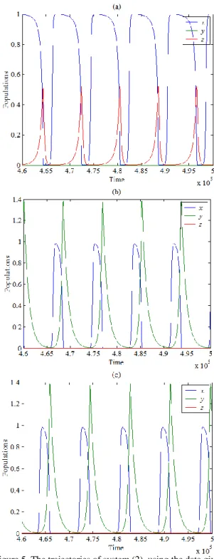
Clearly, Figure 1 shows that the trajectories of system (2) for different initial points approached to the same periodic attractor at different positions. Now, for different values of with other parameters as in Eq. (25), system (2) still persist at periodic dynamics in interior of but with different attractors depending on the value of as shown in Figure 2.

Figure 2. The trajectories of system (2), using the data given

by Eq. (25) with respectively, approach

asymptotically to periodic attractors in interior of

Clearly, as shown in Figure 2, increasing causes decreasing in infected prey and predator

but the system still approaches to periodic attractor in interior of . Now, varying the value of in the ranges and with the rest of parameters as in Eq. (25) leads to extinction in and respectively and the trajectory of system (2) approaches asymptotically to periodic attractor in the interior of plane and plane respectively. Otherwise, the system still approaches to periodic attractor in the interior of , see Figure 3 for typical values for . It is observed, the parameters and have similar effects, but with different ranges, as those obtained for

.

Figure 3. The trajectory of system (2), using the data given by Eq. (25) with different values of , approaches asymptotically to periodic dynamics in the boundary planes: (a) -Time series of trajectories of system (2) for ,

which approach to periodic attractor in plane; (b) - Time series of trajectories of system (2) for ,

which approach to periodic attractor in plane

It is observed that, varying the value of in the ranges and with the rest of parameters as in Eq. (25) leads to extinction in and respectively and the trajectory of system (2) approaches asymptotically to periodic attractor in the interior of plane and plane respectively. Otherwise, the system still approaches to periodic attractor in the interior of , see Figure 4 for typical values of . Similar results have been

(13)

obtained in case of varying the parameter , but with different ranges as those got for .

Figure 4. The trajectory of system (2), using the data given by Eq. (25) with different values of , approaches asymptotically to periodic dynamics in the boundary planes:

(a) -Time series of trajectories of system (2) for , which approach to periodic attractor in plane; (b) - Time series of trajectories of system (2) for ,

which approach to periodic attractor in plane

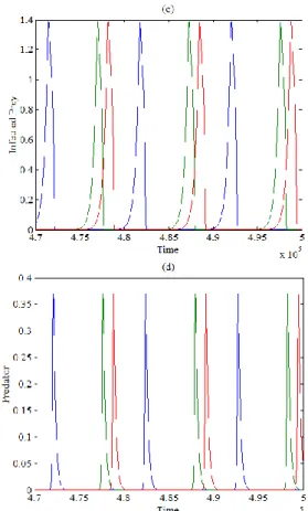
On the other hand, varying the parameters values of , and in the ranges , and respectively, keeping the other parameters as in Eq. (25) leads to approach asymptotically to periodic attractors in the interior of plane, plane and plane too. Otherwise, the system still approaches to periodic attractor in the interior of , see Figure 5 for typical values of , and . Similar results have been obtained in cases of variance of the parameters and as those obtained in case of , and respectively.

Figure 5. The trajectories of system (2), using the data given by Eq. (25), approach asymptotically to periodic dynamics

in the boundary planes: (a) - Time series of trajectories of system (2) for , which approach to periodic attractor in plane; (b) - Time series of trajectories of

system (2) for , which approach to periodic attractor in plane; (c) - Time series of trajectories of

system (2) for , which approach to periodic attractor in plane

Increasing the Allee rate , keeping the other parameters as in Eq. (25), causes extinction in the predator species and the trajectory of system (2) transfers from periodic dynamics in the interior of to periodic dynamics in the interior of the plane. However, increasing the Allee rate, in the case of having a periodic attractor in

(14)

the plane, also leads to extinction in the predator species and the trajectory approaches the periodic attractor in the planetoo, which means that increasing Allee rate leads always to extinaction in predator species. (Figure 6).

Figure 6. The trajectories of system (2), using the data given by Eq. (25), approach asymptotically to periodic dynamics in the boundary plane: (a) - Time series of trajectories

of system (2) for , which approach to periodic attractor; (b) - Time series of trajectories of system (2) for

and , which approach to periodic attractor

It seems that the Allee rate has extinction effects on the predator species and that the system then loses its persistence.

It is observed that, although increasing the value of in the range , keeping other parameters fixed at Eq. (25), satisfies the local stability condition (11c) of the axial equilibrium point , the trajectory of system (2) still asymptotically approaches the periodic attractors in the interior of . This is due to the nonexistence of an initial point in the basin of attraction of the axial point. However, decreasing the value of below the value of 0.51 together with extends the basin of attraction of the axial point so that the initial point (0.75,0.6,0.5) belongs to it, and then the trajectory asymptotically approaches the axial equilibrium point as shown in Figure 7.

by Eq. (25) with and , approach

asymptotically to axial equilibrium point : (a) -Time series of trajectory of susceptible prey; (b) - Time series of trajectory of infected prey; (c) - Time series of trajectory of

predator

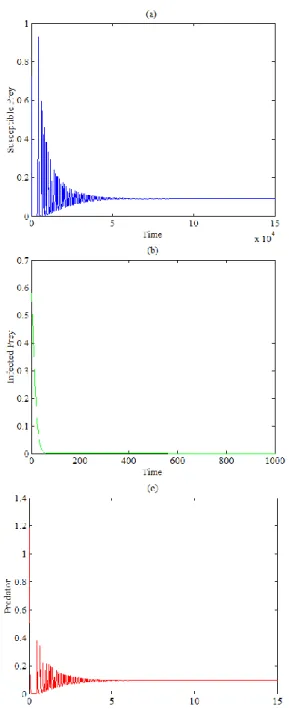
Finally, decreasing the value of below 0.07 with , keeping other parameters as in Eq. (25), causes the trajectory of system (2) to asymptotically approach the infected prey-free equilibrium point in the interior of plane as shown in Figure 8.

(15)

by Eq. (25) with and , approach

asymptotically to infected prey equilibrium point : (a) - Time series of trajectory of susceptible prey; (b) - Time series of trajectory of infected

prey; (c) - Time series of trajectory of predator

VI. C

ONCLUSION

In this paper, a mathematical model considering the Allee effects on the prey-predator system in case of the existence of disease and refugee in prey species is proposed and studied. The properties of the solution of the mathematical model, including existence, boundedness and uniqueness, are discussed. All the possible equilibrium points are found. The local, as well as global, stability for these equilibrium points are investigated. The local bifurcation conditions, including Hopf bifurcation, around each equilibrium point are

also established. It is observed that the proposed model has a rich dynamic and many of its parameters represent bifurcation parameters for the system. Finally, the numerical simulations of the system, with the help of the hypothetical set of data given by Eq. (25), have been shown in different types of dynamics, which can be summarized as follows:

1. The system has different types of attractors including periodic attractor and point attractor.

2. For the data given in Eq. (25), the system has a globally asymptotically stable periodic dynamic.

3. Although increasing the intensity of competition of infected prey to susceptible prey leads to a decrease in the density of infected prey and predator, the system still approaches the periodic dynamics in the interior of .

4. Increasing the contact rate above a specific value (similar to the natural death rate of the predator , the harvesting effort , the available portion of the prey for predation ) causes extinction of the predator species and the system approaches asymptotically to periodic dynamics in plane. However, decreasing below a specific value (similar to , , ) leads to extinction in infected prey and the system approaches asymptotically to periodic dynamics in plane. Otherwise, the system still persist at a periodic dynamics in the interior of .

5. Increasing the inhibitor of disease spread rate above a specific value (similar to an inhibitor harvest rate of the predator ) causes the extinction of the infected prey species and the system approaches asymptotically to periodic dynamics in plane. However, decreasing below a specific value (similar to ) leads to the extinction of the predator and the system approaches asymptotically to periodic dynamics in plane. Otherwise, the system still persists at a periodic dynamics in the interior of .

6. Increasing the attack rate of predator to susceptible prey above a specific value (similar to the conversion rate of the susceptible prey to predator ) causes the extinction of the infected prey species and the system approaches asymptotically to periodic dynamics in plane. However, the system still persists at a periodic dynamics in the interior of .

7. Increasing the half-saturation constant above a specific value (similar tothe preference rate of infected prey ) causes the extinction of the predator species and the system approaches asymptotically to periodic dynamics in

(16)

plane. However, the system still persists at a periodic dynamics in the interior of .

8. Decreasing the attack rate of predator to infected prey below a specific value (similar tothe conversion rate of infected prey to predator ) causes the extinction ofthe predator species and the system approaches asymptotically to periodic dynamics in plane. However, the system still persists at periodic dynamics in the interior of .

9. Increasing the value of the death rate of infected prey above a specific value, so that the local stability condition of the axial equilibrium point is satisfied with decreasing the value of the conversion rate of susceptible prey to predators below a specific value, causes extinction in both the infected prey and predator and the system approaches, asymptotically, the axial equilibrium point.

10. Decreasing the availability portion of prey for predation below a specific value, so that the local stability condition of the infected prey free equilibrium point is satisfied with decreasing the value of the conversion rate of susceptible prey to predators below a specific value, causes extinction in the infected prey and the system approaches, asymptotically, the infected prey free equilibrium point.

11. Finally, increasing the value of the Allee effects causes extinction in the predator species and the system approaches, asymptotically, the periodic dynamics in the interior of the plane. In fact, the trajectory of system (2) transfers from periodic in the plane to periodic in the plane by increasing the value of the Allee effect above a specific value.

R

EFERENCES

[1]

VENTURINO,

E. (2016)

Ecoepidemiology: A more comprehensive

view

of

population

interactions.

Mathematical

Modelling

of

Natural

Phenomena, 11 (1), pp. 49-90.

[2] ANDERSON, R.M. and MAY, R.M.

(1980) Infectious diseases and population

cycles of forest insects. Science, 210 (4470),

pp. 658-661.

[3] BERETTA, E. and KUANG, Y. (1998)

Modeling and analysis of a marine

bacteriophage

infection.

Mathematical

Biosciences, 149 (1), pp. 57-76.

[4] CHATTOPADHYAY, J. and ARINO, O.

(1999) A predator–prey model with disease

in the prey. Nonlinear Analysis, Theory,

Methods and Applications, 36 (6), pp.

747-766.

[5] BAIRAGI, N., ROY, P.K., and

CHATTOPADHYAY, J. (2007) Role of

infection on the stability of a predator–prey

system with several response functions – a

comparative study. Journal of Theoretical

Biology, 248 (1), pp. 10-25.

[6]

BHATTACHARYYA,

R. and

MUKHOPADHYAY, B. (2010) On an

eco-epidemiological model with prey harvesting

and predator switching: local and global

perspectives. Nonlinear Analysis: Real World

Applications, 11 (455), pp. 3824-3833.

[7] BOB, W., GEORGE, A.K., and

KRISHNA, D. (2011) Stabilization and

complex dynamics in a predator-prey model

with predator suffering from an infectious

disease. Ecological Complexity, 8, pp.

113-122.

[8] LIU, X. (2011) Bifurcation of an

eco-epidemiological model with a nonlinear

incidence rate. Applied Mathematics and

Computation, 218, pp. 2300-2309.

[9] NAJI, R.K. and MUSTAFA, A.N. (2012)