近畿大学学術情報リポジトリ

全文

(1)Mem. School. B.O.S. T. Kinki University No.4: 13--22 (1998). 13. Optimization for Property Distribution of Largely" Deformed Slender Members Using Discrete Models Kazuo Yamamoto Abstnlct This paper describes optimization analyses of one-dimensional flexible structures for space application, which make large bending deformation at stowed configuration during the launch. The one-dimensional structural member is modeled by multi rigid bodies and compliance elements. Optimization problems were solved constructing the objective functions concerning the displacement and constraint conditions for the entire volume under setting the radius of the" member as the design parameters. 1 . Introduction We have a method utilizing the large elastic deformation for the stowage of deployable space structures. For example, this method" has been applied to the bar antennas boarded on the initial spacecraft and the foldable parabola antenna reflectors on the recent communication satellites. This type of deployable-stowable structure has the merit that the mechanism can be relatively simple. On the other hand, precise control of structural properties should be necessary in order to realize the effective deployment and stowage function. An attempt of optimization for the stowed configuration in the severe weight limitation is one example. Many studies have been made for the optimization of structures; but they are almost for the linear theory based upon the small deformation. Studies that constitute the optimization problems in consideration with the large geometrical deformation are quite little as far as the authors are informed. In this study examinations by the numerical simulation are made for the determining method of structural parameters which optimize (minimize) the displacement or configuration of stowed condition focusing on the represe~tative slender foldable members. The formulation and analysis by the nonlinear finite element method are general for the large deformation of slender members (1). But, for the reason of easiness and foresight of the analyses the multi-body system which consists of rigid bodies and compliance elements is employed (2). Optimum problems are composed and analyzed numerically with the external radius as the design parameters, the displacements or deformed shape as the objective functions, and the total volume or the minimum radius of the member as the constraint conditions. The steepest descending method is employed for the interactive search of optimum solutions by use of the computer. 2. Description of the model In the large deformation of slender structural members the bending deformation Department of Intelligent Mechanics, Kinki University, Wakayama 649-6493, Japan.

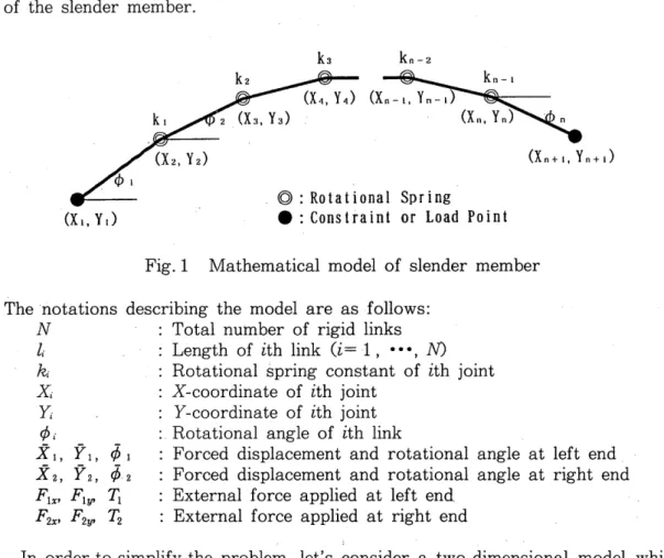
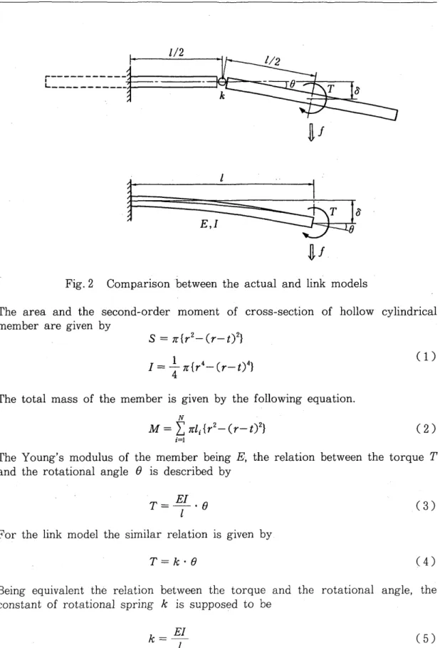
(2) 14. Memoirs of The School of B.O.S.T. of Kinki University No.4 (1998). will be remarkable compared with the axial or shear deformation. Consequently, the multi-body model {rigid body and rotational spring model) shown in Fig. 1 is employed as the mathematical model which simulates the bending deformation of the slender member.. (X n + I, Yn + I). © : Rotational Spring Constraint or Load Point. (XI, YI). .:. Fig. 1. Mathematical model of slender member. The notations describing the model are as follows: N Total number of rigid links li Length of ith link Ci = 1, ••• , N) ki Rotational spring constant of ith joint Xi X-coordinate of ith joint Yi Y-coordinate of ith joint if> i Rotational angle of ith link Xl, Y 1, if> 1 Forced displacement and rotational angle at left end X 2, Y 2, if> 2 Forced displacement and rotational angle at right end FIx, FlY' TI External force applied at left end F 2x , F 2y• T2 External force applied at right end In order to simplify the problem, let's consider a two-dimensional model which deforms only within the plane of paper. The model. consists of N rigid links each of which. is constrained mutually at both ends in the translational direction. At the joint which connects adjacent two links a rotational spring which generates the torque proportional to the angle difference of the two links is equipped. At the left and right ends of this link system, the boundary conditions that constrain the translational and rotational directions. In the unconstrained directions the external loads (translational force and rotational torque) are given. It is necessary to relate the link length and rotational spring' constant with the actual physical properties of the slender member. Fig. 2 shows a comparison between the actual slender member and the link model. The slender member is supposed to be a hollow cylindrical structure with constant external radius rand thickness t in the range of length l. This is called the actual model. Being fixed completely. the left end of the actual model (corresponds to the center of left link), the translational force F or the torque T is applied at the right end of actual model (corresponds to the center of right link). The translational. displacement or rotational angle of the right end is made equivalent between the actual model and the link model..

(3) 15. l/2 ~-----------,~----------~~ ___________ ~~=--=. IL. ~-----------~. ~f Fig. 2. Comparison between the actual and link models. The area and the second-order moment of cross-section of hollow cylindrical member are given by S = 7L{r2- (r- t)2}. 1=. ~ 7L{r 44. ( 1) (r- t)4}. The total mass of the member is given by the following equation. N. M =. L: 7L1i {r2- (r- t)2}. (2). i=l. The Young's modulus of the member being E, the relation between the torque T and the rotational angle (J is described by T= E1 .8 l. (3). For the link model the similar relation is given by T= k· 8. (4). Being equivalent the relation between the torque and the rotational angle, the constant of rotational spring k is supposed to be (5).

(4) 16. Memoirs of The School of B.O.S.T. of Kinki University No. 4 (1998). Being equivalent the relation between the translational force and the translational angle, the rotational spring constant k can be obtained by k=~ EI 4 l. (6). There is some differ~nce between the two cases. It should be evaluated according to the characteristics of the problem (which is essential the translational displacement or the rotational displacement) which case can be selected, because every relations can not be equivalent in the equivalent model. In the present study the latter is employed.. 3. Formulation of equilibrium equations Now, derive the equilibrium equations of this link structure system. The strain energy of the entire system U is given by the following equation. N-l. U = i~. 1. 2. ki( ¢>i+l - ¢>i)2. (7). In each link, following geometrical relations exist between the rotational angle and the coordinates of both ends.. l';-l-l';-lisin¢> = 0. Ci. (8) =. 1, .•. , N-l). The constraint conditions at both ends of the link system are described as follows;. X1-X1=O Y1-i\= 0 ¢>1-¢1=0. 0 YN+l- Y2 = 0 ¢>N+l - ¢ 2 = 0. XN+I-X 2 =. (9). where the symbols with the top bar give the forced displacement and the forced rotational angle, and the suffixes 1 and 2 show the left end and the right end respectively. Equations (8) and (9) are summarized as follows. (0). The equations governing the deformation are described by the energy stationary conditions with constraint equations as follows; (1).

(5) 17. where {qj} is unknown vector defining the location of connecting points, Ak (k = 1 , ••• , 2 N + 6), {fd being the Lagrange'.s multipliers and the external force vector. {qj} = {Xl' ~, 1>1,000, X N + 1, YN + 1 }. Vi}. = {Ft, FlY' T1, 0,000, T2, FfHl' F:+ 1}. Combining the Eq. (1) and (0) simultaneously, (5 N+ 8) nonlinear equations are obtained for (5 N + 8) extended unknown variables qj and Ak We can solve numerically this nonlinear equations system by use of the iterative procedure such as the Newton-Raphson method [ 3 ] considering appropriate initial values near the true solution. 4. Optimization of property and its procedures. There are various parameters for the property which distributes in the longitudinal direction of the sender cylindrical member such as external radius (r), thickness (t), Young's modulus(E) and so on. Now, the external radius is selected as the design parameter for optimization. Consequently, the other parameters are kept unchanged throughout the member. The external radius is related to the rotational spring constant through the second-order moment of cross-section. The entire N---; 1 rotational springs are divided equally into M groups, in which the spring constant, consequently the external radius, has the same value. The design parameters for optimization are defined as the external radius 7k' (k = 1,···, M).. 4 . 1 Conditions for Optimization As the objective function for optimization, 1) the square sum of the displacement in arbitrary direction of the member and 2) the square sum of the deviations of deformed shape of the member from the given shape are considered. For the case 1), the objective function E~bj is defined as the following equation. p. L(xjcos O+Yj sin 0)2. E;bj =. (12). j=l. The condition, that the entire volume of the member is constant, is employed as the constraint condition. In this case, the optimum solution can not be found without this constraint condition. M. L rk-Mro = k=l. °. (13). Furthermore, the external radius of each group has the minimum value rmin .. For the case 2), the objective function E;bj is defined as the following equation; N+I. E;bj =. L F(xj , Yj)2. j=l. (15).

(6) 18. Memoirs of The School of B.O.S.T. of Kinki University. No. 4 (1998). where F(x, y) "is the polynomial which gives the specified shape. In this study the second-order polynomial is employed as follows. (16). In this case, the optimum solution can be obtained without the constant volume condition because the deformed shape to be attained is given definitely. But, the case with this condition is also examined. M. L rk-Mro =. 0. (17). k=l. Similarly to case 1), the external radius of each group has the mInImum value. (18). 4 . 2 Procedures for the search of optimum solution trhe steepest descending Inethod is employed in searching the optimum solution. The objective function EObj is the function of the design parameter 1£, and the direction for the steepest descending without any constraint condition is expressed by gra deE obj ( 1£ )) -. 8E obi. 8 1£. (19). This vector is obtained numerically by the following equation;. (20) where D is the small increment of 1£. When the constraint condition exists, the direction for the steepest descending grad (E obj ) , is the normal projection of grad (E obj ) to the plane of constraint condition as shown in the following equation (4); .)' = d" (E .) _ grad(Eobi ) on gradeE ob'} gra ob'} non· n. (21). where n is the normal vector of the constraint plane. The modification of the design parameters by the steepest descending method IS done interactively according to the following equation.. (22) This means that the search is made in the direction of the steepest descending along the plane of constant volume constraint by giving an appropriate value to A bit by bit, and the value of A is found so that grad(Eobj ) may become extremely.

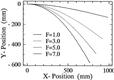
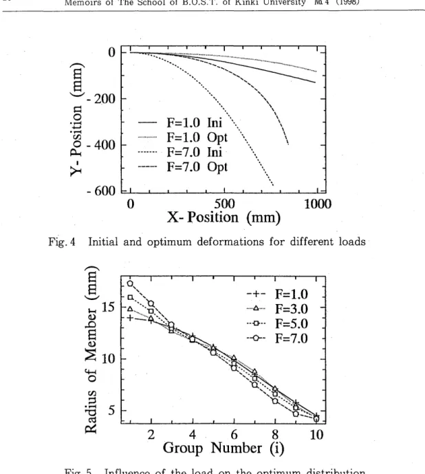
(7) 19. small. A new direction of steepest descending grad (E Obj ) , is calculated at that point. If the design parameter 1£ violate the minimum radius condition in the course of search, calculations hereafter is carried out putting the segment of grad (E obj ) for the parameter as zero. When the absolute value of grad(Eobj ) becomes sufficiently small, the calculation is stopped.. 5. Numerical examples and Disccussion The optimization analyses were carried out for the slender member with the length L = 1000mm, the number of bodies N = 101, the number of groups M = 10, the Young's modulus E=925.6 kgf /mm 2 , the thickness t= 1 mm, the initial external radius ro = lOmm. In the case that the lateral load is applied at the right end of the slender member which is completely fixed at the left end, the external radius distribution was obtained so that the lateral displacement (() = 7[ / 2) at the right end may be minimized. The deformations of the slender member with uniform· external radius (the initial value) are shown for various amount of lateral loads in Fig. 3 .. o. S. E. '-' - 200 ~ o. F=1.0 F=3.0 F=5.0 F=7.0. .~. ~. .~. rJJ. 0-400. Poe I. ~. o. 500. 1000. X- Position (mm) Fig. 3. Nonlinearity of deformations. The nonlinearity of deformation becomes large with increase of the load. For maximum load (F=7.0 kgf) the displacement of the tip is about 60% of the total length of the member. In Fig.4 the deformations are illustrated for both the uniform and the optimum distribution of the external radius in case of the minimum load and the maximum load. In both cases the displacement for the optimum radius distribution is reduced to about 70% of that for the uniform distribution. The optimum radius distribution for various lateral loads is shown in Fig. 5. The larger is the nonlinearity of the deformation, the larger the reduction of radius toward the right end and the larger the increase of radius near the fixed point is. In all cases the minimum radius rmin is set to 4 mm, but this constraint condition does not become active..

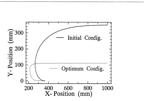
(8) 20. Memoirs of The School of B.O.S. T. of Kinki University No. 4 (1998). o. ,-...... ........~~.~~~.~~::::=:.:.~.~=~.~. . . . . . . . . . . . . . . . . . . . . . . . . . . . . .. S S. .. F= 1.:· · ~:;· \ . """'\\. '-" - 200 o ~. ' .... .. .~. ~. \. .~. en. F=1.0 Opt \\ F=7.0 Ini \,. 0-400. ~ I. F=7.0 Opt. ~. \. \\\. -600~·~~--~~~~~~~--~. o. 500. 1000. X- Position (mm) Fig. 4. Initial and optimum deformations for different loads ,-...... S S '-" ~. Q.). -+- F=1.0. 15. ..·..A .... •• -G ••. ~. S. --0--. Q). ::E. F=3.0 F=5.0 F=7.0. 10. 4-1. o. 2. 4. 6. 8. 10. Group Number (i) Fig. 5. Influence of the load on the optimum distribution. In the case that the forced displacements it 1 = 370mm, Y 1 = 0 mm, ¢ 1 = 7[ rad at the left end and it 2 = 1000mm, ¢ 2 = 0 rad at the right end are applied, the external radius distribution was obtained so that the lateral displacement (() = 7[ / 2) at the right end is minimized. The deformations are depicted for the initial and optimum distribution of external radius of the member in Fig. 6. In the deformed configuration for initial uniform radius the curvature is reduced mildly from the left end toward the right end. On the other hand, for the optimum radius the curvature is large only near the left end and is flat in the right side. The lateral displacement at the right end for the optimum radius distribution is reduced to about 30% of that for the initial radius distribution..

(9) 21. 8 300 e § 200. -. Initial Config.. ""--". ....... .l"'"I • l"'"I. r.n. ~ 100. ............. Optimum Config.. I. ~. 400 600 800 X- Position (mm). 200 Fig. 6. 1000. Initial and optimum deformations. In Fig.7 the convergence toward the optimum distribution of external radius is illustrated. The minimum radius rmin is set to 4 mm. This constraint condition is active in the radius of the third group r3 for the optimum distribution. Obvious change in the radius from the initial uniform distribution can not be seen in the right side region of the member. On the other hand, remarkable changes from increment to reduction are recognized for the radius distribution in the left side region of the member. ",.......... e. I. ~ ~ 20 r- q\\. g. I. ·····6·····. .D',. e (1). =s ~. I '. -+--0--. ~ ~.\\. --0--. \.\. . . . .~. -'V-. \\. I. I. Initial 2nd Iter. 3rd Iter. 4th. Iter. OptImum. o 10 ~+~\t.~+-+6 ........:.*;:;:;~-Q.-Q--Qen &- . . . .t:l............ ...· F. "cr ,.. :=,j. , ••••. o. ;.s. I. ~. 2. C\j. Fig. 7. V. -.--;./' I. f. f. f. 4. 6. 8. 10. Group Number (i). Convergence toward the optimum distribution.

(10) 22. Memoirs of The School of B.O.S.T. of Kinki University No. 4 (1998). 6. Concluding remarks. Relating the simulation for optimization of slender members which are representative foldable structures for space application, following conclusions were obtained. 1 . A method obtaining the equilibrium was proposed that uses the discrete multi-body model for the large bending deformation of the slender members. 2. The optimum distribution for external radius of the slender member that minimize the displacement at the concerned points was solved by the steepest descending method. 3. The proposed optimization procedure was found to be effective through the numerical simulations.. References (1) T. Hisada and H. Noguchi: The Basis and Application of Nonlinear Finite Element Method, Maruzen, 1995. Gn Japanese) ( 2) Kazuo Yamamoto: Simulations of Nonlinear Mechanics, Nikkan-kogyo Press, 1996. Gn Japanese) ( 3) L. C. W. Dixon: Nonlinear Optimization, English Universities Press, 1972. (4) N. Iwahori : Vector Analysis, Shokabo, 1967. Gn Japanese). *~Jf5~ ~ b tJ '5 *Ei3ffl1/3Z*R • JE~:t1i~~ct G*m~tf~*;f~:xf~'c" 1\)(*RB=JjO)~Jf5{lJf5:Jj\~ ~~1~T G t::. ~ O):t1i~r{' 7 ;. -. 7 O)~)Em ,c mJ L -C~fal V. ~. .;J.. v-. V. 3. /. ,C J:. GfiW ~rr"?. t::.o ~Jf5O)~lj{tJTC' tj:" *m~$t;fO)EIHtj'~Jf5,cff§ L -CIililU{*~~5!j~.'t~@]~t~ftlib~ tQQX:G 7( JV7-1' ;f-' T'. -1' .:f: T' Jv~ ffl t, -C)E:r\: L" ~~~)7~Jf50)~-€5- t, :1Jf1E:r\:~ Newton-Raphson m~ ffl t, -C~lj{ t,. t::.o ~~1~:xf~ ~ L -C~~-')EO)cp~pj~:Jj\*m~$*;f~~)E L t::.o ~~:1J[O] 'c?tlfJ L t::.tf~*;f 1~~~~t/'" 7 ;. ~~)E~. Y ~ L L". 1\)(*RB=JjO)*~Jf5'cto tj G~tLct. G ~'tj:~Jf5Jf5tkib~ tQQX: G § I¥JmJ. L" tf~*;ff*f.t-)E{l~;J\wrrmtJ c'O)*Ij~~ftj:O) b ~ ,c~~1~po~@~:t1iQX: L" ~fal~lj{. ~3j<~t::.o ~~~lj{O)~*"ctj:" ~b7°I) ~ 7-1' 7"tJ~~~~~m~1 /7777-1' 7"'cffl~'t::.o ~~t~O)iffi~" m~. L t::.~lj{tfTm • ~*,mib)~5<jJC' ct G L.. ~ ~8jj. tQ ib~ ,C L t::.o.

(11)