JAIST Repository: Blood Flow Simulation System with Interaction between Blood Flow and Blood Vessel Wall using Image Based Cartesian Grid

全文

(1)JAIST Repository https://dspace.jaist.ac.jp/. Title. Blood Flow Simulation System with Interaction between Blood Flow and Blood Vessel Wall using Image Based Cartesian Grid. Author(s). KUMAHATA, Kiyoshi; WATANABE, Masahiro; MATSUZAWA, Teruo. Citation. Journal of Biomechanical Science and Engineering, 3(2): 85-100. Issue Date. 2008. Type. Journal Article. Text version. publisher. URL. http://hdl.handle.net/10119/8503. Rights. Copyright (C) 2008 日本機械学会. Kiyoshi KUMAHATA, Masahiro WATANABE, Teruo MATSUZAWA, Journal of Biomechanical Science and Engineering, 3(2), 2008, 85-100. http://dx.doi.org/10.1299/jbse.3.85. Description. Japan Advanced Institute of Science and Technology.

(2) Journal of Biomechanical Science and Engineering. Vol. 3, No. 2, 2008. Blood Flow Simulation System with Interaction between Blood Flow and Blood Vessel Wall using Image Based Cartesian Grid* Kiyoshi KUMAHATA**, Masahiro WATANABE*** and Teruo MATSUZAWA**** **School of Information Science, Japan Advanced Institute of Science and Technology, 1-1 Asahidai, Nomi, Ishikawa, Japan E-mail: [email protected] ***Fujitsu Limited, 4-1-1 Kamikodanaka, Nakahara, Kawasaki, Kanagawa, Japan E-mail: [email protected] ****Center for Information Science, Japan Advanced Institute of Science and Technology, 1-1 Asahidai, Nomi, Ishikawa, Japan E-mail: [email protected]. Abstract For the simulation of the fluid-structure interaction (FSI) between the blood flow and blood vessel walls, we have examined the voxel-based FSI method. This method uses a Cartesian grid, called voxel, made from medical images. Further, we have tested the accuracy and reliability of this simple method and have observed its features. In this document, we discuss the background, kinetic models of the blood vessel, a numerical method, and the result of an experiment conducted using an artificial identical shape and an actual realistic shape. Key words: Blood Vessel, Cartesian Grid, Voxel, Medical Image, Fluid Structure Interaction. 1. Introduction. *Received 2 Nov., 2007 (No. 07-0678) [DOI: 10.1299/jbse.3.85]. The use of computer-simulation-based approaches in biomechanics has been growing in recent years. Diseases of the circulatory system are one of the leading causes of death in developed countries (1)(2). It is known that diseases frequently occur in the part where the blood flow is disordered (3)(4). This suggests that the kinetic effects of human blood flow on the blood vessel wall are closely related to the onset and aggravation of circulatory diseases. Therefore, nowadays, several blood vessel simulations are performed. Mori (5) studied the effects of aortic arch torsion on the blood flow and Ohashi (6) studied the effects of athero on the blood flow in the coronary artery. Recently, in order to simulate realistic shape of blood vessels, instead of using a simple artificial shape described by a B-spline surface created by using computer aided design (CAD), the use of a complex realistic shape described by polygons reconstructed by an actual patient’s medical images has increased. Here, medical images are obtained using widely used medical diagnosis techniques, e.g., computed tomography (CT) or magnetic resonance imaging (MRI). Watanabe (7) studied the wall shear stress due to the blood flow in an aorta with an aneurysm or disjunction. Oshima (8) studied the wall shear stress caused by the blood flow in the cerebral artery. In these studies, in order to express a realistic blood vessel shape as a computational grid, the reconstruction of the blood vessel surface as a polygon surface and a complicated unstructured grid have been used. However, the surface reconstruction and construction of such a grid is time consuming and requires considerable. 85.

(3) Journal of Biomechanical Science and Engineering. Vol. 3, No. 2, 2008. expertise. Therefore, it is difficult to simulate a realistic blood vessel to assist everyday diagnosis. If the computational grids can be more easily obtained, blood flow simulation will be simplified and it can be of greater assistance in diagnosis and treatment during everyday diagnosis. Nowadays, the use of methods that use a Cartesian structured grid to express computational shapes, called voxel-based methods, is being considered. These methods can directly obtain medical images as a computational grid and they do not require the reconstruction of a blood vessel shape to a polygon surface for obtaining the grid. Such researches have been performed by Matsunaga (9), who studied the 2D blood flow simulation based on voxels, and Yokoi (10), who simulated 3D blood flow in a cerebral artery with multiple aneurysms on the Cartesian grid. Iwase (11) studied voxel-based blood flow simulation for a cerebral artery and Hattori (12) studied the blood flow in a cerebral aneurysm. Decamps (13) studied a carotid artery with stenosis. However, a blood vessel is elastic and this elasticity requires the consideration of fluid-structure interaction (FSI). This interaction is a subject of considerable interest in both medical and engineering fields. Many FSI researches have been performed by using complex unstructured grids for blood, e.g., Christine (14) and Gerbera (15). Meanwhile Lei (16) studied the voxel-based FSI analysis of the flow around a vibration cylinder caused by karman vortex, but it was not for a blood flow Therefore, in order to assist in actual diagnosis and treatment, we studied voxel-based FSI for blood vessels (17)(18). In the subsequent sections, as a report of the result of the early stage of our study, we describe the FSI analysis using simple kinetic models and a basic shape approximation such as the stair-step approximation.. 2. Models of Blood Flow and Blood Vessel Wall In this chapter, we specify the type of blood vessels considered in our study and the assumptions related to the blood flow and blood vessel walls. We considered the artery as an example of a blood vessel because the kinetic effect of the blood flow on the blood vessel wall is stronger for an artery than for a vein. In addition, we considered that the blood vessel diameter ranged from 1.0 mm to 10.0 mm owing to the limitation of the medical image resolution. In general, it is known that the blood flow in an artery with a diameter between 1.0 mm and 10.00 mm can be assumed to be laminar because its Reynolds number is lower than 2000, and it can be assumed to be a Newtonian viscid because its shear rate is lower than 50 s–1 (19). For the flow model of the blood flow, we consider a Newtonian, viscid, incompressible, laminar, and pulsatile flow. Furthermore, the effect of blood cells was excluded because the blood cell diameter is approximately 8× 10–3 mm, which is considerably smaller than the diameter of the blood vessel. The kinetic model of the blood vessel wall considers a homogeneous isotropic elastic medium obeying Hooke’s law that is deformed by the load from the blood flow. In fact, the blood vessel wall is an anisotropic material. Simulations of an anisotropic material require that the principal axes be defined. However, it is difficult to define the principal axis in image-based voxel data. Therefore, we considered the wall to be an isotropic material in this case. In addition, by excluding the thin three-layered structure of a blood vessel that cannot be recognized in medical images due to its thinness and by considering that the blood vessel is monolithic, we employed a simple linear elastic material to model the blood vessel. Furthermore, we excluded the shear force on the wall due to viscosity because we estimated that the shear force is very small as compared to the pressure force (approximately 1% of the pressure force according to Newton’s law of viscosity and the blood flow velocity in the artery.). 86.

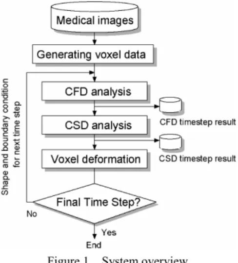
(4) Journal of Biomechanical Science and Engineering. Vol. 3, No. 2, 2008. 3. System Overview In this chapter, we introduce an overview of the FSI analysis system developed in our study. First, we describe the treatment of the FSI in our system. Subsequently, we shall discuss the four major parts of our system. Two methods are mainly used for considering the FSI. One is a weak coupling method and the other is a strong coupling method. The former alternately performs fluid analysis and structure analysis; the result of one analysis is used as input data for another. This method is easy to implement and has great scope for further improvement since the fluid and structure are separately analyzed and each analysis can be independently improved. The strong coupling method solves a simultaneous linear equation that is constructed from the combined discretization of the flow and structure equations. In general, this method gives a higher accuracy as compared to the weak coupling method, but is difficult to improve due to its complicated formulation. We have employed the weak coupling method that alternately solves the fluid and structure problems. Hence, in order to know the interaction between the fluid and the structure, the system alternately performs two analyses. Moreover, to perform a complete analysis, it is necessary to generate a grid and grid deformations. In other words, this system comprises four major parts: generating voxel data, computational fluid dynamics (CFD) analysis, computational structure dynamics (CSD) analysis, and voxel deformation. Figure 1 shows the relationship between these parts. The following subsections describe these parts.. Figure 1. System overview. 3.1 Generating Voxel Data For shape approximation on voxels, there are some approximation levels (20). In the current stage of this study, as the most basic shape approximation for a voxel before progressing to higher approximation levels, we employed the stair-step approximation. This part generates such stair-step voxel data as a computation grid from medical images. There are two steps involved: volume generation and binarization. The first step involves the generation of volume data by stacking sliced images of human CT images. The volume data consists of lots small cubes, called cells (or voxels), that correspond to a pixel in an image. Although actual medical images are grayscale images having more than 255 levels, by performing normalization in advance using the medical image processing software Real INTAGE (21), each cell can be made to have a brightness level ranging from 0 to 255 that corresponds to the original CT values of the human tissues. The second step is volume binarization in which cells are classified as either blood cells. 87.

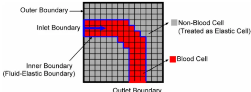
(5) Journal of Biomechanical Science and Engineering. Vol. 3, No. 2, 2008. or non-blood cells by considering the brightness corresponding to the blood brightness in the image as the threshold. Note that in this paper, the term blood cell does not signify “red blood cells” or “cells” as described in biology. Since all the cells are classified as either blood cells or non-blood cells by this step, the blood vessel shape will be approximated by a stair-step. Nowadays, CT images do not have sufficient resolution to distinctly identify a thin blood vessel wall. Therefore, in the current stage of this study, we did not consider thin blood vessel walls. The entire non-blood cell is considered to be elastic, while a blood vessel is considered to be a hole in an elastic brick (similar to a wormhole in a tree). And, the entire region has two types of boundaries. One is the inner boundary between the blood and an elastic medium, while the other is the outer boundary that is the face of the elastic brick. Furthermore, the outer boundary has two more types of boundaries, namely, the inlet and outlet boundaries. Figure 2 shows the shape approximation in a stair-step with two types of cells and all the boundary types.. Figure 2. Stair-step shape approximation using two types of cells and all types of boundaries. The issue of ignoring thin blood vessel walls thickness is expected to be solved by improvements in the CT resolution and with developments in image processing techniques. Hereafter, a blood cell and a non-blood cell is referred to as a fluid cell and an elastic cell, respectively. 3.2 CFD Analysis In this part, we analyze the blood flow behavior in the fluid cell region of voxel data. Since we assumed that the blood flow was Newtonian, viscid, incompressible, laminar, and pulsatile, it could be described by two equations. One is the Navier-Stokes equation Eq. (1) of momentum and the other is the continuum equation Eq. (2), which is a conservation law. Here, u , p, and Re denote the velocity vector, pressure, and Reynolds number, respectively. Equations (3)–(5) are boundary conditions. Equation (3) shows the pressure Dirichlet boundary condition at the outlet boundary and p is a pressure Dirichlet value that is zero. Equation (4) gives the pressure Neumann boundary condition at the inner boundary and n is the normal velocity of the boundary. Equation (5) gives the velocity Dirichlet boundary condition at the inlet boundary and the inner boundary. u denotes the velocity Dirichlet value that is defined to be the corresponding velocity value at the inlet boundary and zero at the inner boundary on initial time step.. ∂u 1 2 + u (∇ ⋅ u ) = −∇p + ∇u ∂t Re. (1). ∇ ⋅u = 0. (2). p = p on ∂p = 0 on ∂n. S p _ diriclet S p _ neumann. (3). (4). 88.

(6) Journal of Biomechanical Science and Engineering. Vol. 3, No. 2, 2008. u =u. on. Su _ diriclet. (5). The fluid analysis of the blood flow was performed by the HSMAC method using voxels in a staggered grid. In this grid, velocity is located on the boundary of the fluid cell and pressure is located at the center of the fluid cell. In HSMAC method, the time advance of velocity and pressure are solved as follows. The velocity predictor of time n+1 at time n is defined as Eq. (6) from Eq. (1) using the Euler explicit scheme.. 1 2 n  ∇u  u~ = u n + ∆t − un (∇ ⋅ u n ) − ∇p n + Re  . (6). Here, ∆t denotes the time splitting. Since the predictor is not the exact value of substitution in Eq. (2) does not yield a zero value.. ∇ ⋅ u~ = ε ≠ 0. u n+1 , its (7). ∇ ⋅ (u~ + δu ) = 0 . Since ε = ε (u~( p)) = ε ( p) , the task of finding δu becomes that of finding δp , which gives ε ( p + δp) = 0 . By the Taylor series expansion of this expression and ignoring the higher-order terms, δp is obtained as below. We should determine. ε ( p + δp) = ε ( p) + δp δp=−. a. δu. value. that makes. ∂ε +… = 0 ∂p. (8). ε ( p) ( ∂ε / ∂p ). (9). The discretization of Eq. (1) by the first-order Euler explicit method for time with implicit n +1 pressure discretization gives the expression for u .. 1 2 n  u n+1 = u n + ∆t − u n (∇ ⋅ u n ) − ∇p n+1 + ∇u  Re  . (10). Subtracting Eq. (6) from Eq. (10) gives. u n+1 − u~ = −∇( p n+1 − p n ) = −∇δp ∆t Because. (11). ∇ ⋅ u n+1 = 0 from Eq. (2), the divergence of Eq. (11) is. ∇ 2δp =. ε 1 ∇ ⋅ u~ = ∆t ∆t. (12). The discretization of Eq. (12) using the central difference for ∇ and changing it to diagonal dominance leads to the expression for the pressure corrector δp : 2. 89.

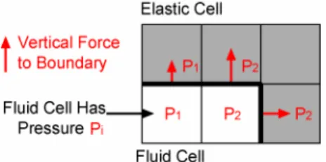
(7) Journal of Biomechanical Science and Engineering. Vol. 3, No. 2, 2008. δp = −. ε. (13).  1 1 1  2∆t  2 + 2 + 2  ∆y ∆z   ∆x. ∆x , ∆y , and ∆z represent the grid size (voxel size). The velocity corrector δu = u − u~ is obtained from Eq. (11) as below.. Where. n +1. δu = − ∆t∇δp. (14). = u + δu , will be obtained by calculating δp and The velocity of time step n+1, u δu alternately until ε is nearly equal to zero. In order to compute the velocity predictor Eq. (6), we employed the fractional-step method with the CIP scheme for the advection 2 term and the central difference scheme for the terms with ∇ and ∇ . The convergence –4 criteria of ε was 1.0 × 10 . n +1. n. 3.3 CSD Analysis In this part, we analyze the behavior of the elastic cell region under a flow pressure resulting from a surface force. Since we assumed that the blood vessel wall was a homogeneous, isotropic, and elastic medium obeying Hooke’s law, the blood vessel obeys the balance equation Eq. (15) (22), kinematical boundary condition Eq. (16), geometrical boundary condition Eq. (17), and the relation between displacement and strain Eq. (18). Moreover, we employed Eq. (19) as the constitutive equation for the linear elastic medium. Let us consider that σ ij is the stress, ρg i is the body force, ni is normal to the surface, and t i is the surface force; in our kinetic interaction model, this surface force causes the blood flow pressure. Blood flow pressure is assigned to the boundary of the fluid cell and elastic cell vertically, as shown in Fig. 3.. Figure 3. Vertical force to fluid-elastic boundary. Moreover, d i is the degree of freedom of the displacement vector of the blood vessel wall and d i is the boundary condition of the forced-displacement vector of the blood vessel wall. St and S d represent the kinematical boundary and geometrical boundary, respectively. ε ij is the strain, E is Young’s modulus, and ν is Poisson’s ratio.. ∂σ ij ∂xi. + ρgi = 0. σ ij ni = ti di = di. on. (15). St. on S d. 1  ∂d. ∂d . ε ij =  i + j  2  ∂x j ∂xi . (16) (17). (18). 90.

(8) Journal of Biomechanical Science and Engineering. Vol. 3, No. 2, 2008.   1   ν  σ xx   1 −ν    ν  σ yy   σ  E − ν ( 1 ) zz  1 −ν  =  σ xy  (1 + ν )(1 − 2ν )  0      σ yz  σ   0  zx    0  . ν. ν. 1 −ν. 1 −ν. 0. 0. 0. 0. 1. 0. 0. 0. 0. 1 − 2ν 2(1 − ν ). 0. 0. 0. 0. 1 − 2ν 2(1 − ν ). 0. 0. 0. 0. ν. 1. 1 −ν. ν 1 −ν.    0  ε xx     ε yy  0   ε  zz  0  ε xy     ε yz  0  ε   zx   1 − 2ν  2(1 − ν )  0. (19). The structure analysis of the elastic cell region in the blood vessel was based on the FEM displacement method (22) using the voxels as hexahedral elements. We consider σˆ ij that satisfies Eq. (15) and Eq. (16) and the displacement dî that satisfies Eq. (15) and Eq. (17). Using dî as a weight, we transform Eq. (15) to the weighted residual form. ˆ  ∂σ ij d i dV = 0  ρ g + i ∫V  ∂xi . (20). Applying the Gauss divergence theorem to Eq. (20) gives Eq. (21).. ∫ σ ij. V. ∂dî dV = ∫ ti dî dSt + ∫ niσ ij d j dSu + ∫ ρg i dî dV ∂x j St Sd V. Now, if we also consider virtual displacement. ∫ σ ij. V. δd i , Eq. (21) becomes Eq. (22).. ∂ (dî + δd i ) dV = ∫ ti (dî + δd i )dSt + ∫ niσ ij d j dSu + ∫ ρgi (dî + δd i )dV ∂x j St Sd V. Subtract Eq. (21) from Eq. (22) and consider boundary condition.. ∫σ. ij. V. (21). ∂δdi dV = ∫ tiδd i dSt + ∫ ρg iδd i dV ∂x j St V. δdi = 0. on. Sd. (22) by the geometrical. (23). From Eq. (18),. 1  ∂δd i ∂δd j  δε ij =  + 2  ∂x j ∂xi . (24). Using Eq. (24) and Eq. (23) yields. ∫ σ δε ij. V. ij. dV = ∫ tiδd i dS t + ∫ ρg iδd i dV St. (25). V. Equation (25) is called the principle of virtual work. Here, by denoting the stress tensor as {σ } and the strain tensor as {ε } , the constitutive equation Eq. (19) becomes {σ } = [ D]{ε } . The principle of virtual work becomes. 91.

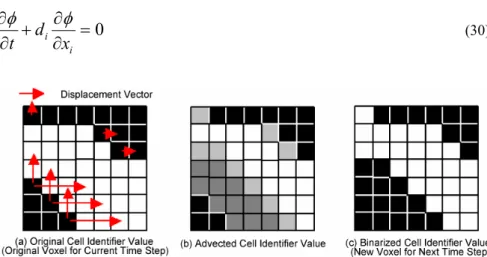
(9) Journal of Biomechanical Science and Engineering. Vol. 3, No. 2, 2008. T T ∫ δ {ε } {σ }dV = ∫ δ {d } {t}dSt + ∫ δ {d } {ρgi }dV T. V. St. (26). V. Here, {ρg i } is the gravity force vector. Furthermore, the displacement {d } is e interpolated as {d } = [ N ]{d } in an element (e), where [N ] is the interpolation e function in the element and {d } is the node displacement vector of the element (e). {ε } e is written as {ε } = [ B ]{d } . Therefore, Eq. (26) becomes. [ K ]{d } = {F }. (27). [ K ] = ∑ ∫ [ B]T [ D][ B]dVe. (28). e Ve. {F } = ∑ ∫ [ N ]T {t n }dS te + ∑ ∫ [ N ]T {ρg i }dVe e Ste. (29). e Ve. In Eq. (28) and Eq. (29), ∫Ste and ∫Ve imply the integration on an element and refers to the summation of all elements. Here, {tn } is the equivalent nodal force that ∑e replaces the surface force. By solving Eq. (27), the displacement corresponding to the pressure is obtained. In order to solve Eq. (27), we employ the ICCG method and set the convergence criteria as 1.0×10–6. Further, we ignore the effects of gravity. 3.4 Modifying Shape and Boundary Condition for Next Time Step This part involves a modification in the shape of the fluid cell region and the boundary condition for the next time step. First, with regard to modifying the shape, since voxels comprise the Eulerian grid, unlike the Langragian grid, a grid point cannot be moved to express the entire shape deformation because all the grid points are fixed in the Eulerian grid. In general, to express the shape deformation, the Eulerian method solves the mass or density (or the other degree of freedom) advection equation. In other words, the fluid-structure boundary is flowed in the Eulerian grid. This system also involves the solving of the advection equation to express the deformation of the blood vessel wall. The quantity to be advected is the cell identifier value. This value is defined by whether the cell is fluid or elastic. If the cell is fluid, the value is 255, and if the cell is elastic, the value is 0. In other words, an original identifier value that is the value before solving the advection equation is either 255 or 0. This part solves the cell identifier value advection equation Eq. (30) by using the first-order upstream difference scheme, where φ is the cell identifier value and d i is the blood vessel wall displacement computed in the CSD analysis part. Figure 4(a) shows the original identifier value and the displacement vector.. ∂φ ∂φ + di =0 ∂t ∂xi. Figure 4. (30). Steps for generating new voxel data for next time step. 92.

(10) Journal of Biomechanical Science and Engineering. Vol. 3, No. 2, 2008. After solving the advection equation, the identifier value is distributed in the range of 0 to 255, as shown in Fig. 4(b). These smoothed identifier values are used as the input data in generating the voxel data part. The generating voxel data part again generates voxel data through binarization, as shown in Fig. 4(c). In the shape model of this step, since the shape is expressed in the form of a stair-step by two types of cells, namely, fluid cells and elastic cells, the effect of a displacement smaller than the voxel size will not affect the fluid analysis in the next time step. In order to involve the effect of a small displacement, as a velocity boundary condition for fluid analysis, the wall displacement velocity u is assigned on the boundary between the fluid and non-fluid, as shown in Fig. 5. Here, the wall displacement velocity u is defined as u = d ∆t , where u is the Dirichlet boundary value of velocity in Eq. (5), d is the resultant displacement in Eq. (27), and ∆t is the time splitting.. Figure 5. Moving wall boundary condition. 4. Numerical Experiment In order to estimate the performance of our voxel-based FSI method, we performed FSI analysis of a straight elastic cylindrical tube deformation under pulsatile inflow. Moreover, we generated voxel data for a realistic coronary artery from the medical image of an actual patient. We performed FSI analysis for the deformation. 4.1 Straight Elastic Cylinder Tube For comparison with this method, which uses a conventional-boundary-fitted unstructured grid, we performed the analysis for a simple shape. The simulated shape was the elastic cylindrical tube shown in Fig. 6. The tube had a length and inner diameter of 100 mm and 10 mm, respectively.. Figure 6. Elastic tube under pulsatile flow. As a fluid analysis condition, we assumed that the fluid was blood. Its density was ρ =1.0 g/cm3 and the viscosity coefficient was µ =0.035 poise. The inlet condition was a uniform flow that pulsated with time. The time profile of the pulsatile flow had the shape of a sine function, as shown in Fig. 7, with a cycle of 1.0 s and a peak Reynolds number of 100. The pressure P was 0 at the outlets. The wall was assumed to be a non-slip wall. As a structure analysis condition, the Young’s modulus of the wall was 1.0 MPa and Poisson’s ratio was 0.3. A constraint condition was assumed in that the outer boundary is fixed for all directions.. 93.

(11) Journal of Biomechanical Science and Engineering. Vol. 3, No. 2, 2008. Figure 7. Inlet pulsatile flow velocity. First, to determine the extent to which the analysis region size affects the result, we performed an experiment by changing the elastic brick size. In this experiment, the voxel resolution was 1 mm and the brick length was 100 mm. Since the width and height are equal, they are represented as the breadth, the value of which ranges from 20 mm to 100 mm in steps of 10 mm. Figure 8 shows the specifications of the elastic brick. The time splitting ∆ t was 0.01 s. The analysis was performed using a PC with an AMD OpteronTM 2.4 GHz processor and 4 GB memory. The computation time was a maximum of 7764 s for 1 pulsatile cycle.. Figure 8. Figure 9. Specifications of elastic brick. Radial displacement corresponding to the breadth. Figure 9 shows the maximum radial expansion displacement corresponding to the different breadths. It indicates that the displacement becomes smaller with a decrease in the brick breadth in the breadth range of less than 60 mm. Next, we compared our voxel-based code with a consumer FSI software FIDAP (23) using the same test case. In this experiment, the elastic brick breadth of 100 mm was used for voxel. Further, a computational grid was prepared for FIDAP using a conventional grid-making software called GAMBIT (24) from the CAD model of a tube having a length, inner diameter, and outer diameter of 100 mm, 10 mm and 16 mm, respectively, i.e., the elastic wall thickness was 3 mm. In the FIDAP grid, the averaged ∆ x was 1.0 mm. Figure 10 shows the radial displacement distribution of the cylinder for the maximum expansion and shrinkage of the cylinder. In this figure, the horizontal axis represents the length along the cylinder axial direction length and the vertical axis represents the radial. 94.

(12) Journal of Biomechanical Science and Engineering. Vol. 3, No. 2, 2008. displacement. Figure 10(a) shows the maximum-expansion displacement distribution when the cylinder expands through the pulsation cycle. It indicates that the expansion peak was located on the part immediately following the inlet in the case of both voxels and FIDAP. In FIDAP, the resulting maximum displacement was of the order of 1.6×10–4 mm, but in voxel the result was 2.0×10–5 mm (very low.) Figure 10(b) shows the maximum-shrinkage displacement distribution when the cylinder shrinks through the pulsation cycle. It indicates that the shrink peak was also located on the part immediately after the inlet in both cases. In the FIDAP result, the maximum displacement order was –1.2×10–4 mm, but in the voxel result, it was –2.0×10–5 mm (very low.). (a) Maximum expansion (b) Maximum shrinkage Figure 10 Two types of maximum radial displacement. In the cases of both expansion and shrinkage, a significant feature was observed that the displacement in the voxel result was lower than that in the FIDAP result. We thought that the cause of this feature was the stair-step approximated boundary and the fact that the wall thickness was ignored by considering the elastic tube to be a hole in an elastic brick as mentioned previously. In order to avoid the stair-step approximated boundary, we plan to improve the boundary to a better approximation level (20). Further, if the image resolution will be sufficiently improved in the future to enable the recognition of thin blood vessel walls, the issue of ignoring the wall thickness can be avoided. This feature showed the same tendencies for different Young’s modulus values of 0.25, 0.50, 1.00, 2.00, and 4.00 MPa. The ratio of the radial displacement of voxels to the radial displacement of FIDAP was 13.78% on an average during expansion, and 14.96% during shrinkage, as shown in Fig. 11. The average of both expansion and shrinkage was 14.37%.. Figure 11. Ratio of voxel resultant displacement to FIDAP resultant displacement. According to this feature, when we used a Young’s modulus of 143.7 KPa, that is, 14.37% of 1.0 MPa, a good aspect of displacement that corresponds to the FIDAP result of 1.0 MPa was obtained, as shown in Fig. 12.. 95.

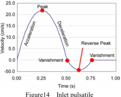
(13) Journal of Biomechanical Science and Engineering. Vol. 3, No. 2, 2008. (a) Maximum expansion (b) Maximum shrinkage Figure 12 Two types of maximum radial displacement using 143.7 KPa for voxel. In this case, the voxel code estimated the elastic wall to be harder as compared to the FIDAP. However, the aspect of the deformation was well simulated. Therefore, we thought that if such a displacement feature is apparent in a simple pre-examination, the voxel-based code could be used for an easy analysis in everyday diagnosis. 4.2 Actual Blood Vessel We performed FSI analysis for the blood vessel using actual CT images of patients. Diseases with high mortality rates such as cardiac infarction and angina pectoris occur due to coronary artery diseases. Therefore, as a sample of an actual and complex blood vessel shape, we employed the coronary artery.. Figure 13. Coronary artery. The simulated shape was the left main coronary trunk shown in Fig. 13. The diameter of the inlet part A was 0.481 cm. In this figure, the part from inlet A to end B is the main coronary trunk, the part from Branch 1 to end D is the 1st diagonal branch, and the part from Branch 2 to end C is the 2nd diagonal branch. In this case, the 1st diagonal branch had mild stenosis in the bent part located around the right side of Fig. 13. Moreover, the 2nd diagonal branch and the main coronary trunk also have mild stenosis after Branch 2. The raw CT images are “Digital Imaging and COmmunication in Medicine (DICOM) (25) ” image data—211 sheets of sliced images of 512 × 512 pixels of the heart and its surrounding areas. The size of the image was set as 15 cm × 15 cm × 10 cm. The image resolution was 0.0293 cm/pixel and 0.0474 cm/sliced image. Since the original CT images have regions that are unnecessary for the analysis and the slice image resolution differs from the pixel resolution, we removed the unnecessary region and adjusted the resolution to be constant at 0.0344 cm in all directions using the medical image processing software Real INTAGE (21). Further, the tube was also treated as a hole in an elastic brick. The voxel data obtained from this set of adjusted medical images comprised a 98×106×40 cell. In the fluid analysis condition, the fluid considered was blood. Its density was ρ =1.0 g/cm3 and the viscosity coefficient was µ = 0.035 poise. The flow at the inlet was a pulsatile flow, as shown in Fig. 14. Its cycle was1.0 s and the peak Reynolds number was 300. Pressure was zero at the outlets of B, C, and D in Fig. 13. The wall was considered to be a non-slip wall.. 96.

(14) Journal of Biomechanical Science and Engineering. Vol. 3, No. 2, 2008. Figure14. Inlet pulsatile. As a material property, we employed a Young’s modulus of 143.7 KPa and Poisson’s ratio of 0.3. Inlet end A and outlet ends B, C, and D were fixed in all directions as a constraint condition because outer boundary was fixed. The analysis was performed using PC having an AMD OpteronTM 2.4 GHz processor and 4 GB memory. The computation time was a maximum of 116115 s for 1 pulsatile cycle. Although this computation time was larger than one day, it may be improved in the future since this code is still under development. Figure 15 show the aspects of the flow velocity at particular times t=0.125, 0.250, 0.375, 0.500, 0.625, and 0.750 s during a pulsatile flow. In these figures, to facilitate clear observations, the density of the drawn flow velocity vector is half. The vector length and color have been defined by assuming the maximum velocity value as 84.6 cm/s. At t=0.125 s, the middle time of the inflow acceleration term, although a major part of the blood flow was in the main coronary trunk, some part of the blood flow was in both the diagonal branches. In the stenosis part of the diagonal branch, there was a high velocity. At t=0.250 s, which is the peak time of the inflow acceleration term, there was an increase in the velocity corresponding to the inflow increase in the main coronary trunk and the 1st diagonal branch. However, in the 2nd diagonal branch, there was no significant difference in the velocity from t=0.125 s. At t=0.375 s, the middle time of the inflow deceleration term, there was no significant decrease in the velocity observed in the main coronary trunk. However, in both the diagonal branches, there was a significant decrease in velocity. In particular, in the 2nd diagonal branch, there was negligible blood flow.. t=0.125 s. t=0.250 s. t=0.375 s. t=0.500 s. t=0.625 s Figure 15 Flow velocity. t=0.750 s. 97.

(15) Journal of Biomechanical Science and Engineering. Vol. 3, No. 2, 2008. At t=0.500 s, the time for the absolute recession in the inflow velocity, the flow in the main coronary trunk significantly decreased. Further, in the two diagonal branches, there was negligible blood flow. At t=0.625 s, the peak time of the reverse inflow, the flow ceased in the main coronary trunks, and the two diagonal branches. An extremely small reverse flow appeared in the inlet part. At t=0.750 s, the time for the subsequent absolute recession in the inflow velocity, a slightly high reverse velocity was observed in the inlet part. However, we thought that it was caused by an instantaneous discontinuous change in the inflow velocity in the pulsatile wave used by us, similar to the water hummer phenomenon. Figure 16 shows the aspects of the blood vessel wall displacement vector at particular times at t=0.125, 0.250, 0.375, 0.500, 0.625, and 0.750 s during a pulsatile flow. In this figure, to facilitate clear observation, the density of the flow velocity vector drawn is half. However, unlike the velocity in Fig. 15, the vector length and the vector color have been defined as a maximum displacement value in each time instant because the degree of displacements were significantly different. At t=0.125 s, the middle time of the inflow acceleration term, the part immediately preceding Branch 1 was decreased. The maximum displacement length was 7.56 × 10–4 cm. At t=0.250 s, the peak time of the inlet acceleration term, the part immediately preceding Branch 1 continued to decrease. Further, the part between Branch 1 and Branch 2 in the main coronary trunk also decreased. The maximum displacement length was 1.80 × 10–3 cm. At t=0.375 s, the middle time of the inflow deceleration term, the deformation was similar to that at t = 0.250 s, and the part immediately preceding Branch 1 and the part between Branch 1 and Branch 2 in the main coronary trunk continued to decrease. The maximum displacement length was 4.10 × 10–3 cm.. t=0.125 s. t=0.250 s. t=0.375 s. t=0.500 s. t=0.625 s t=0.750 s Figure 16 Wall displacement (In order to observe the vector clearly, each figure has an individual vector length and color map). At t=0.500 s, the time for the absolute recession in the velocity, the part immediately preceding Branch 1 was increased. The maximum displacement length was 8.14 × 10–3 cm. At t=0.625 s, the peak time of the reverse inflow, a slightly complicated aspect was observed in the deformation. The part immediately preceding Branch 1 expanded. However, the part immediately preceding Branch 2 in the main coronary trunk and the 1st diagonal branch contracted. Hence, the maximum displacement length was too small, 5.82 × 10–5 cm, with no significant deformation observed.. 98.

(16) Journal of Biomechanical Science and Engineering. Vol. 3, No. 2, 2008. At t=0.750 s, the time of the inflow velocity vanished again, and the part immediately preceding Branch 1 and the part between Branch 1 and Branch 2 expanded. The maximum displacement length was 4.74 × 10–3 cm. Through the pulsatile flow, the two diagonal branches had no deformation. We thought that the kinetic effect on the blood vessel wall from the blood flow was low because the velocity change was small in both the diagonal branches, as shown in Fig. 15.. 5. Summary In this study, we have developed an analysis system that can easily use a Cartesian structured grid of the blood vessel shape from medical images without the reconstruction of the blood vessel shape into complex polygons, which requires considerable expertise. In addition, the kinetic interaction between the blood flow and the blood vessel wall is important for the onset and aggravation of circulatory system diseases. We employed basic assumptions for the kinetic models of the blood flow and the blood vessel wall, and a simple approximation for the shape expression, e.g. stair-step approximation. Nonetheless, we were able to confirm that the system could qualitatively simulate the resulting wall deformation of kinetic interaction between the blood flow and the blood vessel wall in a limited condition by comparing it with conventional methods using a simple test case. Owing to this study, despite the complicated shape of the blood vessel, advanced knowledge on the construction of a computational grid is not required. Therefore, even a person who is not an expert in computational simulations can perform the FSI analysis for the blood vessel in 3D. Further, we plan to improve the boundary so that instead of a stair-step approximation, a better approximation can be used.. References (1) (2). (3). (4) (5). (6). (7). (8). (9). Japan Ministry of Health, Labour and Welfare, Summary of Vital Statistics, Trends in leading causes of death, 2006. U.S Department of Health and Human Services Centers for Disease Control and Prevention, National Center for Health Statistics, Health, United States 2006, pp.191-192.(1) No Reference. Glagov.S, Zarins.C, Giddens.D.P, Ku.D. N, Hemodynamics and atherosclerosis. Insights and perspectives gained from studies of human arteries. Arch. Pathol, Lab. Med. Vol.112, pp.1018-1031. 1988. Schievink WI, Intracranial Aneurysms, N engl J Med, Vol.336, pp.28-40. 1997. Daisuke Mori, Takami Yamaguchi, Computational Fluid Dynamics Analysis of the Blood Flow in the Thoracic Aorta on the Development of Aneurysm, J. Jpn. Coll. Angiol, Vol.43: pp.94-97, 2003. Tsuyoshi Ohashi, Hao Liu, Takami Yamaguchi, Blood Flow And Coronary Atherosclerosis -A Computational Mechanical Analysis-, Proc. Conf. on Computational Engineering and Science, Vol.5, No.2, pp823-824. 2000. Masahiro Watanabe, Teruo Matsuzawa, Computational Simulation of Flow in a Dissecting Aortic Aneurysm Reconstructed from CT Images, Proceedings of ISCT: 5th International Symposium on Computational Technologies for Fluid / Thermal / Chemical Systems with Industrial Applications, ASME 2004. Mari Oshima, Kiyoshi Takagi, Motoharu Hayakawa, Toshio Kobayashi, Numerical Simulation and Visualization of Blood Flow in Cerebral Arteries, Journal of Visualization Society of Japan, Vol.22, No.85, pp.77-81. 2002. Nami Matsunaga, Hao Liu, Ryutaro Himeno, An Image-Based Computational Fluid Dynamic Method for Haemodynamic Simulation, JSME International series C, Vol.45, No.3, pp.989-996, 2002.. 99.

(17) Journal of Biomechanical Science and Engineering. Vol. 3, No. 2, 2008. (10) Kensuke Yokoi, Feng Xiao, Hao Liu and Kazuaki Fukasaku, Three-dimensional numerical simulation of flows with complex geometries in a regular Cartesian grid and its application to blood flow in cerebral artery with multiple aneurysms, Journal of Computational Physics, Volume 202, Issue 1, pp.1-19, 2005 (11) Hidehito Iiwase, Ryutaro Himeno, Hideo Yokota, Numerical Multi-scale Analysis of Hemodynamics in a Cerebral Artery, Proceedings of the 19th CFD symposium, D8-1 (2005). (12) Kyota Hattori, Ichiro Takahashi, Kenichi Hattori, Shigeru Miyachi, Katsuya Ishii, Computation of Blood Flow in the Cerebral Aneurysm arising from the Bifurcation of the Cerebral Artery, Proceedings of the 2004 Annual Meeting of JSFM, pp.130-131. (13) T. Deschamps, P. Schwartz, D. Trebotich, P. Colella, D. Saloner and R. Malladi Vessel segmentation and blood flow simulation using Level-Sets and Embedded Boundary methods, International Congress Series, Vol.1268, pp.75-80. 2004. (14) Christine M Scotti, Alexander D Shkolnik, Satish C Muluk, Ender A Finol, Fluid-structure interaction in abdominal aortic aneurysms: effects of asymmetry and wall thickness, BioMedical Engineering OnLine 2005, 4:64 doi:10.1186/1475-925X-4-64. (15) J.F.Gerbeau, M.Vidrascu, P.Frey, Fluid-Structure interaction in blood flows on geometrics based on medical imaging, Computers and Structures Vol.83, pp.155-165, 2005. (16) Kangbin Lei, Masako Iwata, Ryutaro Himeno, Simulation of Fluid-Structure Interaction Using Voxel Method, Transactions of the Japan Society of Mechanical Engineers, Series A, Vol.70, No.691, pp.434-441, 2004. (17) Kiyoshi Kumahata, Masahiro Watanabe, Teruo Matsuzawa, Fluid-Structure Interaction Simulation for Blood Vessel using 3D Voxel Data Derived from Medical Image, Proceedings of FEDSM2007 / 5th Joint ASME/JSME Fluids Engineering Conference. FEDSM2007-37576, 2007. (18) Kiyoshi Kumahata, Kazuhiro Noguchi, Masahiro Watanabe, Teruo Matsuzawa, Voxel Based Simulation for Blood Flow and Blood Wall Interaction Using Image of Medical Treatment, Theoretical and Applied Mechanics Japan, Vol.55, pp.271-278, 2006. (19) Toshio Kobayashi ed., Handbooks of Computational Fluid Dynamics (in Japanese), (2003), pp.667, Maruzen Co., Ltd. (20) Kenji Ono, Product Design using Cartesian Mesh Method, Journal of Japan Society of Fluid Mechanics, Vol.21(2002), pp.16-25. (21) http://www.kgt.co.jp/feature/realintage01 (22) JSME, Computational Mechanics Handbook, Vol.1, 1998, pp.10-12. (23) http://www.fluent.com/software/fidap/index.htm (24) http://www.fluent.com/software/gambit/index.htm (25) http://medical.nema.org. 100.

(18)