Robust H
∞
Control for Active Magnetic Bearing System
with Imbalance of the Rotor
2012SE024 Masaki GOTO Supervisor Gan CHEN
1
Introduction
In this paper, H∞ controller is designed to suppress the vibration caused by the static and dynamic imbal-anced rotor and gyroscopic effect. The purpose of this study is to control attitude of the rotor by state feed-back. Mathematical model of AMB has the first and the second order terms of the angular velocity of the rotor. In attempt to guarantee the robust stability for a prescribed range of angular velocity with lower con-servativeness, the second order terms are changed into first order terms by using linear fractional transforma-tion (LFT) and descriptor representatransforma-tion. Polytopic representation is applied to the system matrices which has the first order terms of the varying parameter. H∞ controller is derived by solving a finite set of LMI condi-tions at vertex matrices. Furthermore the effectiveness of the proposed controller is illustrated by the simula-tions comparing with robust linear quadratic controller (RLQ).
2
Modeling
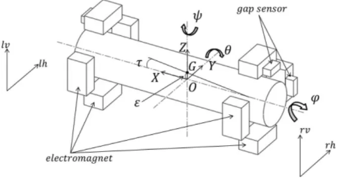
AMB has four electromagnets and two gap sensors at the both ends of the rotor. The perturbations from equi-librium point are derived by the variable transformation after the models are derived at coordinates of X, Y and
Z. The coordinates X, Y and Z are set as shown in
Figure 1. The origin point of the coordinates is the
ge-Figure 1 AMB system
ometric center of the rotor. gj[m] is the perturbation of
gap from equilibrium point. Constant current of elec-tromagnet and controlled input are represented by Ij
and ij, respectively (j = {lv, rv, lh, rh}). The suffices
mean as follows, lv is vertical direction of the left side,
lh is horizontal direction of the left side, rv is vertical
direction of the right side, and rh is horizontal direction of the right side, respectively. To control attitude of the rotor, the current of the electromagnets are adjusted. Physical parameters of AMB are shown in Table 1. The rotor has both static and dynamic imbalance as shown in Figure 1. Here, distance between the geometrical cen-ter and the cencen-ter of gravity of the rotor is represented as ε. Angle between the geometrical axis and inertia
Table 1 physical parameters
parameter symbol unit
Acceleration of gravity g [m/s2]
Mass of rotor m [kg]
Length of rotor lm [m]
Distance between the center and
the center of gravity of the rotor ε [m]
Angle of the rotation axis to inertia axis τ [rad]
Distance between the center of gravity
and the left side of the electromagnet lml [m]
Distance between the center of gravity
and the right side of the electromagnet lmr [m]
Moment of the X axis Jx [kgm2]
Moment of the Y axis Jy [kgm2]
Steady-state value of the sensor G [m]
Suction force constant k [Nm2/A2]
Radius of rotor r [m]
Constant current of vertical direction Ilv, Irv [A]
Constant current of horizontal direction Ilh, Irh [A]
Bias current B [A]
axis is represented as τ . The force and torque caused by the imbalance are occurred in equation of the motion as follows [1]. m¨z = flv+ frv− mg + mεp2sin(pt) (1) m¨y = flh+ frh+ mεp2cos(pt) (2) Jyθ = J¨ xp ˙ψ + flvlml− frvlmr+ (Jy− Jx)τ p2sin(pt)(3) Jyψ =¨ −Jxp ˙θ− flhlml+ frhlmr+ (Jy− Jx)τ p2cos(pt) (4) Here, y and z are the displacement in the direction of the axis Y and Z, respectively. θ and ψ are the rotation angle around the axis Y and Z, respectively. p and fj
are the angular velocity and the levitation force of the electromagnets, respectively (j ={lv, rv, lh, rh}). The angular velocity p(t) is treated as a time varying param-eter. z, y, θ and ψ can be approximated by assuming the displacement from steady gap gj(t) are small enough
[2]. The levitation force of the electromagnet is given as Eq. (5) [3]. fj= k { (B + (Ij+ ij))2 (gj− G)2 −(B− (Ij+ ij))2 (gj+ G)2 } (5)
The state variable x(t) and the input variable u(t) are defined as follows.
x(t) = [glv grv glhgrh ˙glv ˙grv ˙glh ˙grh]T (6)
u(t) = [ilv irv ilh irh]T (7)
The state equation of AMB is derived as follows. ˙
LFT is applied to disturbance matrix D(p2). The de-scriptor representation is derived as state-space repre-sentation as follows.
E ˙xl(t) = Al(p)xl(t) + Blu(t) + Dlw(t) (9)
Eq. (9) is equivalent to Eq. (8) but has no second order terms of angular velocity. The range of time varying parameter p is defined as p∈[p, p]=[p1, p2
] .
Matrix Al(p) is represented by the following matrix
polytope.
Al(p) = αAl(p1) + (1− α)Al(p2), α∈ [
0, 1] (10) Robust H∞controller is designed for the system (9) with matrix polytope (10).
3
Controller design
The output zl(t) is defined to design H∞controller as
follows.
zl(t) = Wxxl(t) + Wuu(t) (11)
For the obtained state-space representation Eq. (9), we design the state feedback H∞controller. The LMI con-ditions to derive the state feedback H∞ controller sta-bilizing the system (8) are as given as follows.
Theorem 1 : If there exist matrices X and Y satis-fying the following LMI conditions, the system (9) is stabilized by u = Kxl = Y X−1xl and the system (8)
is stabilized by u = ˜Kx = Y11X11−1x. Furthermore, H∞ norm||Twzl||∞is less than γ∞.
He[M (p)] Dl (WxX + WuY ) T DT l −γ∞2 I O WxX + WuY O −I ≺ 0 (12) M (p) = Al(p)X + BlY, Y = KX (13) X = [ X11 0 X12 X22 ] , X11≻ 0, Y = [Y11 0] (14) To guarantee the stability of the system (9), Eq. (12) have to be satisfied for all p ∈ [p1, p2
]
. However, in-equality (12) has only first order terms of p. If Eq. (12) is satisfied by common solution at the both vertex matrices Al(p1) and Al(p2), the stability is guaranteed for all angular velocity. Common solution is obtained by solving the following set of LMI conditions shown in Corollary 1.
Corollary 1 : If there exist matrices X and Y satisfy-ing (14), (15), the system (9) is stabilized by u = Kxl=
Y X−1xl= ˜Kx = Y11X11−1x for the prescribed range of angular velocity p and||Twzl||∞ is less than γ∞.
He[M (pi)] Dl (WxX + WuY ) T DlT −γ∞2 I O WxX + WuY O −I ≺ 0 (15) (i = 1, 2) The feedback gain K stabilizing the system (8) is derived from obtained matrices X and Y .
4
Simulation
In this section, the effectiveness of proposed method is illustrated by simulations using mathematical model
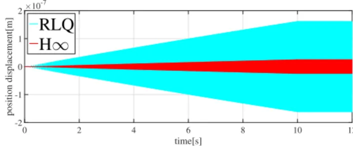
of MBC 500 [3]. The angular velocity of the rotor is in-creased to 25,000 [rpm] in 10 seconds. In this study, the rotor has both static and dynamic imbalance. There-fore, the vibration increase with p2. Note that the dis-turbance itself can not be controlled. In this situation, we aim to suppress vibration as much as possible. The simulation results of the displacements from the equilib-rium point and input current on the vertical direction of the left side are shown in Figure 2 and Figure 3, respec-tively. From Figure 3, the input currents of H∞ and
0 2 4 6 8 10 12 time[s] -2 -1 0 1 2 position displacement[m] ×10-7
RLQ
H∞
Figure 2 The displacement of the rotor on the vertical direction of the left side
0 2 4 6 8 10 12 time[s] -0.1 -0.05 0 0.05 0.1 input current[A]
H∞
RLQ
Figure 3 The input current on the vertical direction of the left side
RLQ are approximately equal. However, from Figure 2, the vibration is suppressed by H∞ control than RLQ. The effectiveness of proposed H∞ control is illustrated.
5
Conclusion
This paper proposes design of a robust H∞controller for AMB system whose rotor has both static and dy-namic imbalance. The proposed controller is designed to suppress the vibration caused by imbalance and gyro-scopic effect. Furthermore the effectiveness of the pro-posed controller is illustrated by simulations comparing with RLQ.
References
[1] H. Seto, T. Namerikawa and M. Fujita, “Exper-imental Evaluation on H∞ DIA Control of Mag-netic Bearings with Roter Unbalance, ” Proc. of the 10th International Symposium on Magnetic Bear-ings, 2006.
[2] W. Shinozuka and T. Namerikawa, “Improving the Transient Response of Magnetic Bearings by the H∞ DIA Control”, Proc. of the 2004 IEEE International Conference on Control Applications, 2004.
[3] Magnetic Moments, L. L. C. “MBC 500 Magnetic Bearing System Operating Instructions”, Magnetic Moments, USA, 1995.