A Numerical Method for Determining the Parameters of Schwarz-Christoffel Transformation

23 Short Report

Kawasaki Journal of Medical Welfare Vol. 17, No. 1, 2011 23-28

Introduction

　In the paper [1] we established a method of the finite element approximation by which we can construct the parallel slit mappings. Parallel slit mapping is a kind of conformal mapping [2, 3] by which we can obtain the exact solutions of partial differential equations expressing physical phenomenons like fluid flows and electric fields in the two-dimensional problems. The purpose of the present paper is to show how to find the exact solutions which can confirm the precision of finite element approximations for the problem having a restricted domain.

　Let zj (j = 1,···,n) be the vertices of polygon Π on the extended z-plane and let ijπ (0 < ij ≤ 2; j = 1,···,n)

be the interior angles of Π. Let w = f(z) be the conformal map of the interior of the polygon Π on z-plane onto the upper half of w-plane: Im w > 0, and let wj (j = 1,···,n) be the points on the real-axis of the w-plane

satisfying wj = f (zj) (j = 1, · · · , n). Then we can state the Schwarz-Christoffel transformation:

　If wj ≠ 3 (j = 1,···,n), it follows that

; dw C C z f 1 w w w w w w w 1 w w n 1 1 2 1 0 2 n 1 _{- g - +} = -= - i- i- i -l ] g

#

] g ] g ] g

and if wn = 3, it follows that

; z f 1 w C w w w w w w dw C 1 n 1 w w 2 1 1 1 1 1 0 n 2 _g = - = - i - i- - i + -- -- _l ] g

#

] g ] g ] g

where C ≠ 0 and C' are complex constants, w0 is a fixed point.

　We note that the Schwarz-Christoffel transformation is written in terms of wj and ij (j = 1,···,n). The

parameters C, C' and wj (j = 1,···,n) of Schwarz-Christoffel transformation can be determined analytically

Abstract

　In the present paper we construct a numerical method for determining the unknown parameters that appear in the Schwarz-Christoffel transformation. For the polygon on the upper half domain with two cuts, we introduce some integrals and their derivatives and obtain the integral formulae which can be easily computed by the numerical quadratures. We show the numerical computations in the cases of d = 1/4, 1/8, 1/12, 1/16 (2d is the distance between two cuts).

(Accepted May 23, 2011)

Key words: Schwarz-Christoffel transformation, polygon, removal of singulality, numerical quadratures

Hisao MIZUMOTO

*

and Heihachiro HARA

*

A Numerical Method for Determining the Parameters of

Schwarz-Christoffel Transformation

*

Deparment of Health Informatics, Faculty of Health and Welfare Services Administration, Kawasaki University of Medical Welfare, Kurashiki, Okayama 701-0193, Japan

for some restricted polygons. In the present paper we construct a numerical method for determining the parameters for the polygon lying on the upper half domain with two cuts. We apply our result to numerical calculations of

d=1/4, 1/8, 1/12, 1/16 (2d is the distance between two cuts). 1. Polygon Πd and conformal mapping

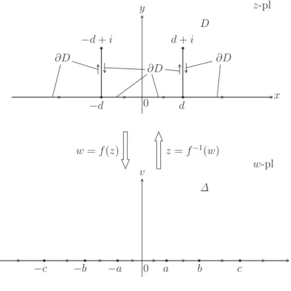
　Let D be the upper half domain with two cuts:

, ,

z x d y z x d y

D="z y; >0,-" ; =- 0< #1,," ; = 0< #1,

on the z-plane]z= +x iy d, >0g, and let ∂D be the oriented boundary of D (see Figure 1). Let Πd be the

polygon D + ∂D.

Fig. 1 Conformal map w = f(z) : D "V

　LetV be the upper half domainV="w v >; 0, on the w-plane w] = +u ivg. For suitably chosen values a, b and c (0 < a < b < c), the domain D can be conformally mapped onto V so that the points: - -d 0, - +d i, - +d 0, d-0, d i d+, +0 and 3 on the z-plane are mapped to the points:

, , , , ,

c b a a b c

- - - and 3 on the w-plane respectively as shown in Figure 1.

　Let w = f(z) be the conformal map: D " V. The conformal mapping of V onto D is given by . z f w w w dw w a c b 1 2 2 2 2 2 2 w 0 = - -- ] ] ] g g g

#

The unknown parameters a, b and c are obtained by solving the following simultaneous equations for a given constant d:

z-pl

D

x

y

−d

0

d

−d + i

d

+ i

∂D

∂D

∂D

w-pl

∆

u

v

−c

−b

−a

0

a

b

c

w

= f (z)

z

= f

−1

(w)

Schwarz-Christoffel Transformation 25 　　　　　　　 　 a b c, , w dw d, a w c w b 1 a 2 2 2 2 2 2 0 / { - -= ] ] ] g g g

#

　　　　　　　 　 a b c, , w a c w b w dw 1 a b 2 2 2 2 2 2 2   / { - -= ] ] ] g g g

#

and 　　　　　　　 　 a b c, , . c w dw w a w b 1 b c 2 2 2 2 2 2 3 / { - -= ] ] ] g g g

#

　The simultaneous equations can be solved numerically by adopting the following iterative procedure: 　(i) Assume the initial values a0, b0 and c0]0 <a0<b0<c0g;

　(ii) Obtain Taj , Tbj and Tcj (j = 1, 2, · · · ) by solving the simultaneous linear equations.

, , , a a b b c c d a b c 1 1 1 1 j 1 j 1 j j 1 j j 3 3 3 2 2 2 2 2 2 { { { { + = -+ ] - - -g , , , a aj b bj c cj 1 aj 1 bj 1 cj 1 2 2 2 2 3 3 3 2 2 2 2 2 2 { { { { + + = - ] - - -g , , , a aj b bj c cj 1 aj bj cj 1 1 1 3 1 1 1 3 3 3 2 2 2 2 2 2 { { { { + + = - ] - - -g 　　　　　　　(j = 1,2,··· ); 　(iii) Compute the modified values aj, bj and cj (j = 1,2,··· ) by

;

, , , ,

aj=aj-1+3aj bj=bj-1+3bj cj=cj-1+3c jj] =1 2 gg

　(iv) Repeat the steps (ii) and (iii) until the following norm becomes smaller than a sufficiently small number f > 0: norm = f12+ +f22 f32<_f, where , , , , , 1, , , d a b c a b c a b c 1 1 1 j j j 2 2 j j j 3 3 j j j f ={ ] g- f ={ ] g- f ={ ] g -　　　　　　 (j = 1, 2,··· ). The values of , a b i i 2 2 2 2 { {

and 2{ (i = 1, 2, 3 ) can be obtained by using the numerical integrations after_2ci the singularities in , a b i i 2 2 2 2 { {

and 2{ (i = 1, 2, 3) are removed. The details of removing the _2ci singularities are shown in the following section.

2. Computation of partial derivatives

　We constructed the formulae for the partial derivatives of {j (a, b, c) (j = 1, 2, 3) with respect to a, b and c.

We only show here the formulae for j = 1 because the another cases (j = 2, 3) are similar to those.

　Firstly, we define integrals F1(m, k) and G1(k) for real parameters k, m (0 < k < m < 1), and modify them to

the forms in which singularities are removed.

　　　　　　F , k ₁ 1_{x 1}x_{k x}2 dx 2 1 2 2 2 0 1 / m m - -] ] ] g g g

#

　　　　　　　　　 f x; , k_{1 x}f21; , k dx 2 f 1; , k, 1 1 0 1 1 m m r m = -+ ] g ] g _{] g}

#

　　　　　　G1 k _{1 x} x_{1 k x} dx 2 2 2 2 0 1 / - -] ] ] g g g

#

　　　　　　　　 ; x ; ; , g x k g k dx g k 1 1 2 1 2 1 1 0 1 1 r = -+ ] g ] g _{] g}

#

where 　　　　　　f x; , k k x , x 1 1 2 2 2 2 1 m / m -] g  x k; , k x x g 1 1 2 2 2 / -] g

　We note that the integrands in these modified forms are finite in the whole range of integration. Thus the values of integrals in F1 and G1 can be obtained precisely by using the numerical quadratures.

　For real parameters k, m (0 < k < m < 1), we define the following partial differentials:

, , , F k kF k _{x k x} x kx dx 1 1 1 1 1 2 2 2 3 2 2 2 2 0 1 2 2 / / m m m - -o _{] ]} ] ] g g g g

#

　Then we have the following formulae for the partial derivatives of {1(a, b, c) with respect to a, b and c.

　　　　　　 _a1 _cb 2 _ba G1 _ca _cb F1 _ba, _ca , 2 2{ = d- d n+ o d nn 　　　　　　 _b1 2 b_c F1 _ba, a_c 2 _ba a_c G1 _ca , 2 2{ _{= d n+ d n 　　　　　　 c}1 b_c F _ba, _ca _ca F _ba, a_c . 2 1 1 2 2{ =-d n d d n+ o d nn

Table 1 Computational results of the polygon Πd

a

_{= 0.106921 × 10}

−2

b

= 0.464919

d

= 1

₄

c

= 1.358104

norm

∗

_<

₁₀

−99

a

_{= 0.131958 × 10}

−5

b

= 0.309317

d

= 1

₈

c

= 1.202315

norm

∗

_<

₁₀

−33

a

_{= 0.195804 × 10}

−8

b

= 0.246405

d

= 1

₁₂

c

= 1.144459

norm

∗

_<

₁₀

−33

a

_{= 0.311939 × 10}

−11

b

= 0.210494

d

= 1

₁₆

c

= 1.113578

norm

∗

_<

₁₀

−32 ∗

_{norm =}

�

_(ϕ

₁

_{− d)}

2

_{+ (ϕ}

2

− 1)

2

+ (ϕ

3

− 1)

2

Schwarz-Christoffel Transformation 27

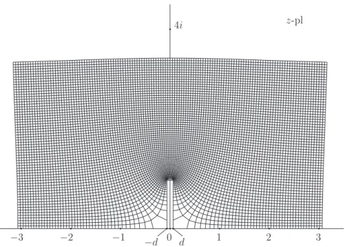
3. Numerical examples

　We obtain a, b and c for the cases of d = 1/4, 1/8, 1/12 and 1/16 of the polygon Πd defined in §1. We

adopted the Gauss method of 128 integration points for obtaining the quadratures appearing in §2. The computational results are shown in Table 1, and the contour lines are shown in Figure 2 (d = 1/4) and Figure 3 (d = 1/16). Since the norms in Table 1 are less than 10-32_{, we can say that our computational}

results are very good.

Fig. 2 Contour lines in the case of d = 1/4; u = ±0.05n, v = 0.05n (n = 0,1,2,···)

Fig. 3 Contour lines in the case of d = 1/16; u = ±0.05n, v = 0.05n (n = 0,1,2,···)

z-pl

−3

−2

−1

−

d

0 d

1

2

3

4i

z-pl

−3

−2

−1

−

d

0

d

1

2

3

4i

Acknowledgements

　The authors are very grateful to the referees for their very helpful comments. References

1. Mizumoto H, Hara H: Finite element method for parallel slit mappings. Jpn J Indust Appl Math 28(2), in print. 2. Driscoll TA, Trefethen LN: Schwarz-Christoffel Mapping. Cambridge, Cambridge University Press, 2002. 3. Henrici P: Applied and Computational Complex Analysis (Vol 3), Wiley Classics Library Edition, New York,