トップ - アジア経済研究所学術研究リポジトリ ARRIDE

The impact of unstable aids on consumption

volatility in developing countries

著者

Kodama Masahiro

権利

Copyrights 日本貿易振興機構（ジェトロ）アジア

経済研究所 / Institute of Developing

Economies, Japan External Trade Organization

(IDE-JETRO) http://www.ide.go.jp

journal or

publication title

IDE Discussion Paper

volume

173

year

2008-10-01

INSTITUTE OF DEVELOPING ECONOMIES

IDE Discussion Papers are preliminary materials circulated to stimulate discussions and critical comments

Keywords: Aid, Consumption Volatility, International Macroeconomics

JEL classification: E32, E21, F35

* Researcher, International Economy Group, Development Studies Center, IDE ([email protected])

IDE DISCUSSION PAPER No.

173

The Impact of Unstable Aids

on Consumption Volatility

in Developing Countries

Masahiro KODAMA*

October 2008

Abstract

In recent years, a large and expanding literature has examined the properties of developing economies with regard to the macroeconomic cycle. One such property that is characteristic of developing economies is large fluctuations in consumption. Meanwhile, aid for the low income countries is extremely volatile, and under certain circumstances, the volatile aid amplifies the consumption volatility. This document examines whether it is possible that the volatile aid yields high consumption volatility in African countries that constitute the majority of the low income countries. Our numerical analysis reveals that the strongly influential aid disbursements yield a considerably large fluctuation in consumption.

The Institute of Developing Economies (IDE) is a semigovernmental, nonpartisan, nonprofit research institute, founded in 1958. The Institute merged with the Japan External Trade Organization (JETRO) on July 1, 1998.

The Institute conducts basic and comprehensive studies on economic and related affairs in all developing countries and regions, including Asia, the Middle East, Africa, Latin America, Oceania, and Eastern Europe.

The views expressed in this publication are those of the author(s). Publication does not imply endorsement by the Institute of Developing Economies of any of the views expressed within.

INSTITUTE OF DEVELOPING ECONOMIES (IDE), JETRO 3-2-2, WAKABA,MIHAMA-KU,CHIBA-SHI

CHIBA 261-8545, JAPAN

©2008 by Institute of Developing Economies, JETRO

No part of this publication may be reproduced without the prior permission of the IDE-JETRO.

The Impact of Unstable Aids on Consumption Volatility

in Developing Countries

Masahiro KODAMA Institute of Developing Economies

ABSTRACT

In recent years, a large and expanding literature has examined the properties of developing economies with regard to the macroeconomic cycle.1 One such property that is characteristic of developing economies is large fluctuations in consumption. Meanwhile, aid for the low income countries is extremely volatile, and under certain circumstances, the volatile aid amplifies the consumption volatility. This document examines whether it is possible that the volatile aid yields high consumption volatility in African countries that constitute the majority of the low income countries. Our numerical analysis reveals that the strongly influential aid disbursements yield a considerably large fluctuation in consumption.

1. INTRODUCTION

In recent years, a large and expanding literature has examined the properties of developing economies with regard to the macroeconomic cycle.1 One such property that is characteristic of developing economies is large fluctuations in consumption. In order to improve the welfare of developing countries, it is very important to acquire a deep understanding of the causes behind the large fluctuations in consumption, since the stability of consumption is closely related to the welfare of the economic agent. Meanwhile, aid for low income countries is extremely volatile, and under certain circumstances, the volatile aid amplifies the consumption volatility. This document examines whether it is possible that the volatile aid yields large fluctuations in consumption in African countries, which constitute the majority of low income countries. Our numerical analysis reveals that the aid disbursement does not have an influence that it is strong enough to account for the high consumption volatility of average African countries. On the other hand, in the cases of certain countries, the aid disbursement causes a considerably large fluctuation in consumption.

The fluctuations in consumption of many African countries are far larger than those of industrial countries. In part, the large fluctuations in consumption are a natural outcome of the large fluctuations in the output of African countries. A simple index that expresses fluctuations in consumption, excluding output fluctuation, is the “relative standard deviation of consumption”; it is calculated as the consumption standard deviation divided by the output standard deviation. Again, in this index again, the values are far larger for the African countries. This research examines the possibility of the volatile aids causing high consumption volatility. 2

Intuitively, it is natural to expect that the timing of aid disbursement, the volatility of aid, and the size of aid affect the degree of fluctuations in consumption.

First, let us take a brief look at the mechanism of how the timing of aid disbursement affects the fluctuations in consumption. If an aid donor provides a resource as aid for an investment, the resource is required to be utilized as the investment. Then the aid recipient government might reduce its ‘own’ spending for the investment, since the investment is increased thanks to the aid, even if the government reduce its own spending for the investment. The reduction in the government self-spending for investment may lead to a reduction in taxes or an increment in subsidies. The tax reduction or subsidy increment raises the disposable income of consumers, which stimulates private consumption. In this case, a part of the given aid for the investment is diverted to private consumption. The diversion of aid to

non-objective use is known as “fungibility.”3 Now we can show that under the presence of the fungibility, the receipt of aid can increase the country’s consumption. Suppose aid is disbursed to an African country in an economic boom and not disbursed in a recession. Even if the recipient country did not receive the aid, the country’s consumption increases because of the increase in income. Under the assumption that the country receives the aid in the economic boom, consumption increases more because of the aid. In a recession, the country’s consumption decreases considerably due to a joint reduction in income and aid. In contrast, let us assume that the aid is disbursed during recessions and not economic booms. In this case, the change in income and aid offset each other. Therefore, the consumption becomes less volatile. In summary, if the timing of aid disbursement is procyclical, an aid recipient country’s consumption becomes more volatile. In contrast, if it is countercyclical, the consumption becomes less volatile.

Second, the mechanism of how the volatility and size of aid influence consumption volatility is rather straightforward. Obviously, a greater amount of aid leads to a greater increase in consumption. Similarly, more volatile aid renders consumption more volatile. We will analyze how much these three elements of aid―timing, volatility, and size― increase the consumption volatility.

The research herein is closely related to preceding researches in the field of aid and consumption volatility. Arellano et al. (2008) are interested in the influence of volatile aid on macroeconomic variables broadly and not on consumption specifically. They develop a dynamic stochastic general equilibrium (DSGE) model that includes a stochastic-aid-shock variable, and compare behavior of the model with and without the stochastic aid. In their simulation without investment adjustment cost, the aid volatility increases the “investment” volatility for the most part. Pallage et al. (2006) examine relationships between the timing of aid disbursement and welfare of the recipient. Instead of constructing a DSGE model, they directly assume the behavior of consumption corresponding to aid disbursement timing, and calculate the recipient’s welfare arising from the consumption.

This research extends the scope of previous projects in three ways. First, our research interest is different from those of authors of the previous studies. In this study, we investigate the research question of to what extent the high consumption volatility of certain African countries can be attributed to volatile aid. To answer the question, we numerically examine the volatile aid’s impact on consumption fluctuation.

Second, on the basis of the DSGE model, we shed light on the effect of aid disbursement on consumption volatility. Arellano et al. (2008) adopt such a model in their research. Assuming a certain single type of aid (an average aid), they compare a

model with and without the “average aid.” By contrast, instead of assuming a single type of aid, we introduce various types of aid by presuming various combinations of aid parameters (the timing of the aid, size of aid, and the volatility of aid) into our model, and analyze how changes in the parameters affect consumption volatility.

Third, we introduce a variable of foreign asset/debt, which is not included in the model of neither Pallage et al. (2006) nor Arrelano et al. (2008). This variable is important for investigations on the influence of aid on consumption fluctuations, since a part of aid shock is absorbed by the change in the variable. Setting the extent of this variable’s change in our model to the actual extent in data, we measure the influence of aid on fluctuations in consumption.

This document is organized as follows. In Section 2 we develop a model. In Section 3 and 4, we present the model’s parameters. In Section 5, first, we show the benchmark simulation result of the model. Second, we investigate the reaction of consumption volatility in response to changes in aid parameters. Finally, in Section 6, we conclude our research.

2. MODEL

Preference. The model used in this paper is a neoclassical dynamic stochastic general equilibrium model. In the economy there are two types of goods: domestic and imported goods.

We assume a representative infinitely lived household. The household maximizes its expected lifetime utility, which is given by

(1)

_∑

( ) ( )

where the parameter β expresses the subjective discount factor of the representative household. γ is a risk-aversion parameter. CD and CM represent domestic goods consumption and imported goods consumption, respectively. θ and 1-θ are weights for CD and CM in the utility function, respectively. l stands for the leisure of the household. The household is given a certain amount of time, which is standardized to unity in this model, and the household distribute the time to leisure (l) and labor (L).

(2) l_t +L_t =1

labor, while η determines the intertemporal elasticity of substitution in labor supply. Production. The domestic good is produced by inputting labor (L) and capital (K).

(3) Y_t =A_tK_t1−αLα_t

In equation (3), A denotes exogenous productivity shocks and Y stands for value added. We postulate that the domestic goods production requires imported intermediate goods, and we presume that both “the ratio between an output and the intermediate goods” and “the ratio between output and value added” are constant. Naturally, in this case, the ratio of the imported intermediate goods to value added is also constant.

(4) mt =μYt

m stands for imported intermediate goods and μ is the ratio between the imported intermediate goods and value added. The reason we include the imported intermediate good in this model is because, in the case of African countries, the amount of imported intermediate good is large and it consists of approximately a half of a whole import, according to GTAP (2003).

The amount of the capital obeys the following law of motion.

(5) t t t t t t K K I I K K _⎟⎟ ⋅ ⎠ ⎞ ⎜ ⎜ ⎝ ⎛ − − + − = + 2 1 ~ 2 ~ ) 1 ( δ φ δ

where δ denotes capital’s depreciation rate. I~ expresses a composite investment. The composite investment is composed of two types of goods: domestically-produced goods (ID) and imported goods (IM). We express the relationship between the three kinds of investments as, (6) ~ =

( ) ( )

In the capital’s law of motion (6), we assume adjustment costs in investment. It is well known that investment simulated from a DSGE model without the adjustment cost tends to become very volatile. The investment volatility strongly affects the consumption volatility of our interest. The resource owned by the household at time t is spent for consumption, investment, or international assets. Thus, when the amount of resource suddenly becomes large (small), if the investment or the international asset also becomes large (small) simultaneously, the amount of consumption becomes stable. This intuition suggests that the investment volatility affects consumption volatility significantly. In order to control the investment volatility at a realistic level in our simulation, we introduce the adjustment cost in investment. In relation to the

formalization of the adjustment cost, we refer to Uribe and Yue (2006).

Budget Constraint, Market clearing conditions, and Shock Process. The representative household in the model faces the subsequent budget constraint.

(7)

(

) (

)

(

)

P expresses a relative price of imported goods in terms of domestic goods. In this research, we consider P to be an exogenous shock variable. There are two types of international financial instruments in the economy. One of them is constituted by the outstanding international debt denoted as B. While Arellano et al. (2008) do not use this variable, we will introduce it into our model. This is because B’s behavior can significantly affects the consumption volatility, as we have seen in the explanation of the investment adjustment cost. Due to the same reason as that behind the introduction of the investment adjustment cost, we introduce the adjustment costs of international borrowing. We adopt a mathematical expression of the adjustment cost used in Schmitt-Grohe and Uribe (2003) as a mathematical expression of the cost. r is the interest rate of the international borrowing. The other international financial instrument is aid, which is denoted as D. In this research, the aid is considered to be a grant aid4, and its disbursement is determined exogenously.

We have two market clearing conditions; one for domestically produced goods and one for imported goods. The former is written as,

(8) Y_t +m_t =C_tD +I_tD +X_t

Care must be taken in writing the left-hand side of the equation. The value on the left-hand side expresses the entire output of domestically produced goods, which is the sum of the value added and intermediate goods. Naturally, domestically-produced intermediate goods can also be added to the left-hand side, but the domestic intermediate good is deleted in the market clearing condition (8), since it appears in the right-hand side as well and the intermediate goods in the both sides are canceled out. The market clearing condition for the imported good is expressed subsequently.

(9) M_t =C_tM +I_tM +m_t

where M stands for the entire amount of import.

We assume that the productivity (A), aid (D), and relative price of the imported good (P) are determined exogenously. The determination process obeys a first-order Markov

process. (10) exp( ) ) exp( ) exp( t t t t t t p P P d D D a A A ⋅ = ⋅ = ⋅ = where ⎥ ⎥ ⎥ ⎦ ⎤ ⎢ ⎢ ⎢ ⎣ ⎡ + ⎥ ⎥ ⎥ ⎦ ⎤ ⎢ ⎢ ⎢ ⎣ ⎡ ⎥ ⎥ ⎥ ⎦ ⎤ ⎢ ⎢ ⎢ ⎣ ⎡ = ⎥ ⎥ ⎥ ⎦ ⎤ ⎢ ⎢ ⎢ ⎣ ⎡ − − − p t d t a t t p d a t t t u u u p d a p d a 1 1 1 0 0 0 0 0 0 ρ ρ ρ , ⎥ ⎥ ⎥ ⎦ ⎤ ⎢ ⎢ ⎢ ⎣ ⎡ p t d t a t u u u ∼N(0,Ω)

The representative household maximizes its lifetime utility given as (1), under the constraints of (2)–(10). We solve this problem numerically with the method of log-linearization.

3. CALIBRATION

The annual subjective discount parameter β is equal to 0.96. The value corresponds to quarterly model’s 0.99 which is often used in RBC literature. The risk aversion parameter γ is set to 2.61, as per Ostry and Reinhart (1992), which econometrically estimates the parameter for developing countries including African countries. We determine the value of θ, the weight parameter between CD and CM, such that the steady-state value of CD/CM corresponds to the average value in the data. We found θ to be 0.89. ψ strongly affects the steady-state level of labor. As per an empirical study by Golin (2002), we select 0.61 as the steady state value of labor supply. η, which governs intertemporal elasticity of substitution in labor supply. In our simulation, η is set to 5.00.

In RBC literature, in reference to α, 0.66 is often adopted, which we also utilize. μ governs the ratio between the value added and the imported intermediate goods in the steady state. GTAP (2003), a type of Input-Output table, reports that the ratio is 0.24. τ determines the ratio between IM and ID in the steady state. GTAP (2003) provides the value of the ratio, and we can replicate the ratio in the steady state by setting τ to 0.517. The capital’s depreciation rate δ is equal to 0.075. φ has a significant influence on investment volatility, and we take advantage of this property of φ, when we replicate investment volatility in our simulation.

ξ corresponds to the steady state value of B. We set the value of ξ/Y so that ξ/Y is equal to the data average of debt outstanding/GDP. ζ determines the burden of B’s adjustment cost, and its magnitude naturally yields a deep impact on the volatility of B, thereby,

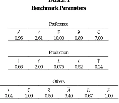
also affecting the volatility of trade balance. We utilize the parameter of ζ in order to replicate the trade balance volatility. r, the interest rate of B, satisfies the following equation in the steady state: β(1+ r)=1. Given β’s value of 0.96, r is equal to 0.04. Table 1 summarizes the calibrated parameters.

TABLE 1

4. SHOCK ESTIMATION

In setting parameters in the shock process, we take two steps: first, following Kose and Riezman (2001), in order to simplify the shock process, we assume a diagonal matrix as the AR(1) coefficient matrix. Second, we estimate the AR(1) process of A, D, and P separately. We adopt estimated ρs and the estimated standard deviation of ua and ud as the parameters in our shock process. In reference to the covariances of ua, ud, and up are assumed in our simulation, and by controlling the size of covariance, we control the correlation between the GDP (Y), the aid (D) and the relative price (P) in our simulation.

In estimating the shock process of a, we adopt the method introduced by Kose and Riezman (2001). Assuming that the fluctuation of capital is rather minimal in the short run, we consider K to be a constant in estimation of a. Using the formula of Solow residual in logarithms, we estimate the Solow residuals. From the Solow residuals, we estimate ρa and the standard error of ua.

Let us now look at the estimation of d. First, we begin with the explanation of the data on aid. We utilize the data on the disbursement and not commitment of aid for aid shock estimation. We exclude the amount of ‘debt relief’ from the aid disbursement data, since, in the case of the debt relief, there is no actual inflow of resource into the recipient country, while we presume the inflow causes the large consumption fluctuation.5 We denote the adjusted aid data by the local currency unit, deflate it with SNA base import deflator, and express it in per capita base.

Second, we estimate the shock process of d, using the real per capita aid. After calculating the logarithm of the per capita real aid, we detrend the logged aid with HP (100). We use the detrended logged real aid for estimation of the shock process.

Similarly, we estimate the shock process of p: We estimate P as the SNA base export price divided by SNA base import price. After calculating the logarithm of P, we detrend the logged P with HP (100). We employ the detrended logged P for the shock

process estimation.

Table 2 presents the estimated shock process parameters.

TABLE 2

5. SIMULATION

Benchmark Simulation. In this section, we analyze our simulation results. First, we examine the benchmark simulation. Second, we compare the benchmark result with other case results wherein we change parameters related to aid disbursement. By means of the comparison, we shed light on our research objective of how much the aid disbursement can amplify African countries’ consumption fluctuations.

We present the major features of macroeconomic fluctuations calculated from the data and the model in Table 3.

TABLE 3

In the table, we display three different types of moments—standard deviation, relative standard deviation, and correlation between GDP and variables. The relative standard deviation of X ― RSD(X) ― stands for the ratio of the standard deviation of a variable X to that of the GDP. The first column includes an index of X/M. While we employ the method of log-linearization, we cannot calculate the logarithm of the conventional trade balance, since the conventional index of X – M representing trade balance can become both negative and positive. Therefore, instead of “X – M,” we utilize X/M as a variable for trade balance.

Before plunging into a detailed analysis of the simulation results, we discuss the features of aid’s moments as calculated from the actual data. The last row of Table 3 displays the aid moments. First, the table clearly shows that the standard deviation of aid is far more volatile than that of GDP. The relative standard deviation of aid is approximately 4.5 times larger than that of the GDP. Pallage and Robe (2003) and many others also arrive at such a finding. Second, the correlation of aid and GDP in the table is slightly negative. However, we have to be careful about this sign. The benchmark case correlation coefficient is only an average of the index of our sample African countries. The size and the signs of the correlation coefficients vary between countries, as we will see in Figure 2 which exhibits the distribution of the correlation coefficients

of our sample African countries. This result is different from the one presented by Pallage and Robe (2001) who concludes that the correlation is positive in most African countries. The difference seems to arise from the difference in the aid data and deflator. We employed aid data that does not include debt relief. Meanwhile, Pallage and Robe (2001) adopted aid that includes debt relief. While we used import deflator for aid data and GDP deflator for GDP data, Pallage and Robe (2001) employed import deflator for both aid and GDP data. Since import deflator is rather volatile, if the two variables are deflated by the import deflator, it is expected that the two deflated variables will have a strong positive correlation sharing the same deflator.

We now proceed to the results of the benchmark simulation. In regard to the standard deviations and the relative standard deviations, generally, our model replicates the data rather well; meanwhile, the standard deviations of consumption and labor are lower than those of the data.

The lower standard deviations of consumption are common to many other RBC researches such as King and Rebelo (1999), which constructs an RBC model for the US and Arellano et al. (2008), which constructs one for developing countries. It is well-known that the presence of durable-good consumption amplifies the fluctuation in consumption significantly. The exclusion of durable goods in the previous studies and our research here decrease the consumption fluctuation of such simulations. On the other hand, the existence of the durable goods will not account for the fact, which is our research interest in this paper, that African countries’ consumption is more volatile than those of the industrial countries. According to Engel’s Law, the share of necessary good consumption of low income countries in their income is higher than that of the high income countries. And the most typical necessary good is food which is not durable. Hence, while the presence of the durable good gives more volatility to the simulated consumption, it will not render the consumption of developing countries in Africa more volatile than those of industrial countries.

The difference in the labor volatility between the data and the simulation originates from the difference in labor concepts. While the simulated labor represents the labor hour, the labor volatility of the data is calculated from the employment statistics because of the availability of data. The empirical literature reveals that the employment labor volatility is higher than the labor hour volatility.

Let now us turn to analyses of the correlation of the variables to GDP. In general, our simulated correlation is higher than the data correlation. In particular, the sign of X/M’s correlation is positive in the data and negative in the model. Nonetheless, this is not a fundamental drawback of our model because of the following rationale: the sign of the

correlation in the data distributes between -0.78 and 0.64 in our sample. This implies that it is not unusual for a correlation coefficient between Y and X/M to be positive. While the average of the correlation coefficients becomes slightly negative in our sample, considering the correlation coefficient’s distribution, it is not impossible that the average may become positive in another sample. Another large difference is the magnitude of L’s correlation coefficient. The difference mainly arises from the data difference which has already been pointed in the explanation of labor’s volatility. While we find such differences in correlation, the model correctly replicate the order of the correlation coefficient size of the GDP components.

Taking such facts into account, we can safely state that, in total, our model mimic the behavior of the African economies rather well.

Sensitivity of Consumption Volatility. In the preceding subsection, we analyzed the benchmark simulation. In this subsection, we change the three aid parameters—correlation between GDP and aid, standard deviation of aid, and the ratio of aid to GDP—and examine the sensitivity of the volatility of consumption with respect to the aid parameters. Table 4 displays the relative standard deviation of consumption for four different simulations.

TABLE 4

Before discussing the results, we explain the items in each row. For the sake of simplicity, hereafter, we denote “standard deviation of a variable X” and “relative standard deviation of a variable X” as SD(X) and RSD(X), respectively. The first row of the table presents the RSD(Aid). The second row exhibits the correlation coefficients between the GDP and aid. The third displays the RSD(C). The differences between the indices denote the differences between the standard deviations of consumption in terms of the standard deviation of the GDP. For example, if the difference between the two cases is 0.084, it implies that the consumption volatility rises, due to the difference in the aid disbursement between the two cases, by 0.084×SD(Y).6 If this was a change in SD(C) and not RSD(C), it would be difficult to judge whether the change was large or small. Therefore, we utilize RSD(C), which stands for the consumption volatility denoted in terms of SD(Y).

The column title “Stable Aid” refers to a case wherein RSD(Aid) is set to zero. The difference between the RSD(C) for “Benchmark” and “Stable Aid” is only 0.05. The result of the small RSD(C) difference proceeds from the value of the benchmark

correlation coefficient which is around zero. This timing of aid disbursement does not amplify the fluctuation in consumption at all. Hence, in order to yield a large RSD(C), we need a considerably large aid-Y ratio, a considerably large RSD(Aid), or a combination of relatively large aid-Y ratio and RSD(Aid). Since the benchmark case is an average case, its aid-Y ratio and RSD(Aid) are not large. Therefore, the difference in RSD(C) between “Benchmark” and “Stable Aid” is small. To summarize, in the case of an average African country the aid does not have a strong influence on consumption such that it can yield large fluctuations in consumption.

The column titles “H. Corr” and “L. Corr” represent the case wherein the aid-Y correlation coefficient is ‘0.5’ and the coefficient is ‘-0.5’, respectively. In Table 4, the difference in the value of RSD(C) between “H. Corr” and “L.Corr” is approximately 0.2. In other words, by changing the aid timing from “L. Corr” to “H. Corr,” the consumption volatility increases by approximately 0.2×SD(Y). Such numbers suggest that the timing of aid disbursement produces non-trivial consumption volatilities in the case of an average African country.

At this point, we are faced with the question of whether the consumption volatility can be considerably amplified by aid that is seemingly influential. The above result tells us that average aid does not produce high consumption volatility. However, it does not mean that the aid does not yield high consumption volatility at all. It is still possible that a seemingly influential aid, not an average aid, cause a large fluctuation in consumption. For this question, we will conduct an experiment: we utilize a combination of the aid parameters, which seems to be more influential in our simulation. Nonetheless, in the following simulations, the combinations of the aid parameters are not completely imaginary but actual ones that were observed in the aid disbursements for certain African countries. The seemingly influential aid-disbursement parameters include those of the outlier countries that are excluded from our sample for the benchmark case, because of their extremely large RSD(C)s. While the values for the RSD(C) for the countries are extremely large, the parameters for the outlier countries other than aid-disbursement and standard deviations are not very different from those of the benchmark case. Table 5 presents the findings of our experiments.

TABLE 5

In the case of “Comoros” in the table, we employ aid disbursement parameters for Comoros in the experiment. Similarly, we refer to the parameters of Gambia and Zambia in “Gambia” and “Zambia.” “Parameter Set I” exhibits the three aid

disbursement parameters: aid-Y ratio, RSD(Aid), and aid-Y correlation coefficient. The effect of aid depends partly on the parameters for P. For example, when the relative price of the imported good (P) is low, if aid is disbursed, then the consumption increases considerably. If the volatility of P is small, the aid-P timing effect on the fluctuation in consumption becomes minimal. “Parameter Set II” presents the parameters of P that affect aid disbursement effects on the consumption volatility.

In the RSD(C) ratio to the benchmark RSD(C), the ratios of “Comoros”, ”Gambia”, and “Zambia” are 1.79, 1.70, and 2.26. Such values are strikingly large. In particular, in the case of “Zambia,” the RSD(C) is more than doubled because of the aid disbursement. Nevertheless, we have to be careful about this index. We underestimated the RSD(C) in our benchmark simulation, in comparison with the RSD(C) in the data. If the underestimation is complemented by the introduction of new exogenous shock variables, the explanatory power of the aid shock with regard to the consumption volatility will fall. Consequently, the above ratio falls. On the other hand, in the case where the underestimation is complemented by a mechanism that amplifies the influence of the present shocks on the consumption volatility (e.g. tighter adjustment cost in the investment, tighter liquidity constraint, durable goods, and so forth) and the mechanism affects neutrally on the shocks, the above ratio keeps the high degree.

At this point, instead of the ratios, we will consider the differences in RSD(C) of our interest and the benchmark case. According to the index, the RSD(C)s of “Comoros,” ”Gambia,” and ”Zambia” increase by 0.38, 0.33, and 0.60, respectively. King and Rebelo (1999) report that the RSD(C) of the US is 0.74. In regard to the RSD(C) of the U.S., the increments in consumption fluctuations are rather significant. In the case of African countries, Cape Verde, Guinea Bissau, Mozambique, and Sao Tome Principe, as well as the above three countries also receive influential aid. If we introduce a new shock variable in order to produce more fluctuation in consumption, it should be the one that does not cancel the effect of the current shock variables on consumption fluctuation. Otherwise, the introduction of the new shock does not increase consumption volatility. Accordingly, even if the RSD(C) ratio falls by the introduction of a new shock variable, the new shock variable does not suppress the differences in the RSD(C) in Table 5, which is considerably large. In summary, we can safely conclude that the effect of the influential aid, such as the ones in Table 5, on consumption volatility is quite considerable.

Next, let us analyze the reaction of consumption volatilities in response to more varied combinations of aid parameters. Keeping the benchmark parameters other than three aid parameters, we change the three aid parameters in Figure 1.

Figure 1

In the figures, we set the ratio of aid/Y to 14.1% and 25%, respectively, where 14.1% is equal to the benchmark parameter value. The basal plane of the figures corresponds to combination of the correlation and relative standard deviation of aid (henceforth, RSD(Aid)). The height of the figures exhibits the RSD(C). Finally, the support of the three parameters corresponds to those of the actual data.

First, we consider how RSD(C) changes in response to RSD(Aid). In the figures, if we go along with the RSD(Aid) axis from zero to fifteen, the edges of the curved surfaces drawn in the figures first descend and then ascend. The mechanism that engenders this phenomenon is as follows. When aid is disbursed countercyclically, the sum of aid disbursement and GDP becomes more stable. To put it differently, the countercyclical aid has the effect of stabilizing the household’s total earning (the sum of aid disbursement, GDP, and the flow of borrowing), which diminishes the RSD(C). On the other hand, if the RSD(Aid) is large, the volatile aid strongly swings the total earning, and the RSD(C) increases. Thus, the edge of the curved surface descends and then ascends. In “Case 2” of Figure 1, the descendent part is shorter, because the ascendant effect is stronger on account of the larger aid/Y parameter.

Second, the figures show that more procyclical aid disbursement timing raises the RSD(C). We have already seen the intuition of the aid disbursement timing’s effect on RSD(C) in the preceding paragraph.

Third, the figures indicate that combinations of high aid-GDP correlation, a large Aid/Y ratio, and high aid volatility produce considerably large RSD(C)s. Further, satisfaction of two of the three elements also yields a relatively large RSD(C). Since the support of the parameters reflects those of the actual data, the maximum values of the parameters are not unrealistically large values. In other words, it is possible that the parameters of aid disbursement parameters take the maximum values of the figures and cause large fluctuations in consumption fluctuations, as evidenced in the cases in Table 5.

At this point, it is worth asking if the data supports our hypothesis that the aid disbursement amplifies the consumption volatility. As evidenced in Figure 1, the standard deviation of aid and the ratio of Aid/Y have a non-monotonous effect on consumption volatility. Further, such effects depend on aid-Y correlation: if the correlation is negative (and if the aid volatility is not extremely large), these two elements have effects that suppress consumption volatility. If the correlation is positive,

these two elements raise consumption volatility. On the other hand, the aid-GDP correlation has a monotonous positive effect on consumption volatility. Moreover, the direction of the correlation’s effect does not depend on the other elements. Since it is easier to empirically identify the monotonous effect on the consumption volatility than the non-monotonous effect in the following data examination, here we focus on the effect of aid-Y correlation. The dots in Figure 2 represent various combinations of RSD(C) and the aid-GDP correlation coefficient that are calculated from the data on African countries.7

Figure 2

As our model predicted in Table 4, the sets of the dots display a positive relationship between the two elements. Such a consequence suggests that the data supports our hypothesis that the aid disbursement timing affects the RSD(C). Further, this supports the validity of our simulation, at least partly.

6. CONCLUSION

The consumption volatility of certain African countries is larger than that for industrial countries. We investigate the effects of the aid disbursement on the large consumption volatility in African countries, by employing a dynamic stochastic general equilibrium model.

On the basis of the model, we examine African economies from several dimensions. First, we confirm that our model can replicate the behavior of the properties of major macroeconomic variables.

Second, we utilize the model to examine how much the different combination of aid disbursement causes further fluctuations in consumption. We find that in an average case, if the timing of aid disbursement is changed in such a way that aid-GDP correlation coefficient changes from –0.5 to 0.5, the relative standard deviation of consumption is raised by approximately 20% of the standard deviation of the GDP. Meanwhile, the average aid, wherein the aid-GDP correlation coefficient is set approximately to zero, does not yield a high consumption volatility. Further, we measure the effect of what appears to be strongly influential aid disbursement. Consequently, we found that in special but realistic cases the aid disbursement has a rather strong effect on the relative standard deviation of consumption: the simulation

suggests a possibility that in the case of countries that experience influential aid disbursement, the consumption volatility can be doubled by way of aid disbursement.

Third, we examine the effect of aid disbursement on consumption fluctuation more comprehensively, by considering various combinations of the three aid-disbursement parameters. We find that in the three parameters for aid disbursement, aid/GDP ratio, aid volatility, and aid-GDP correlation, if at least two of them are quite large, the aid disbursement causes large fluctuations in consumption.

Fourth, we confirm that our simulation is supported by the data for African countries. The data tells us that there is a positive relationship between the aid-GDP correlation coefficient and consumption volatility. This is consistent with our prediction which is based on our dynamic stochastic general equilibrium model.

This paper suggests an important policy implication for the stabilization of consumption: an appropriate policy that stabilizes the volatility in consumption naturally depends on the cause of the consumption volatility. For example, suppose a large-consumption-fluctuation country where the high consumption volatility is caused not by liquidity constraint but by the volatile aid. It will not be productive to introduce policies that decrease the liquidity constraint, as consumption stabilization policy without specifying the source of high consumption volatility. Thus, for the appropriate consumption stabilization policy, we have to clarify the causes that yield a large volatility in consumption in the country. This paper shows that a strongly influential aid is one of the causes of the large consumption fluctuations.

FOOTNOTES

1. Aguiar and Gopinath (2007), Arellano et al (2008), Kose (2002), Kose and Riezman (2001), Mendoza (1995), Neumeyer and Perri (2005), Pallage and Robe (2001), Pallage et al. (2006), Uribe and Yue (2006) and several others have studied the macroeconomic cyclical properties of developing countries.

2. In reference to the role of capital inflow to developing countries, Neumeyer and Perri (2005) argued that the countercyclical interest rates on foreign debts can account for various cyclical properties, including large consumption fluctuations that are characteristic of developing countries. However, we do not adopt the countercyclical interest rate in this research. This is because the portion of debt in the capital inflow to the poorest countries such as African countries is rather small, while the portion of aid is large.

4. Pallage et al. (2006, p.461) presume that most of the non-grant aid is eventually not repaid. We also adopt this assumption.

5. As the aid data, we employed the publicly announced OECD data: we refer to “Net ODA disbursements minus Net debt relief” of OECD’s data.

6. SD(Y) also changes according to changes in aid disbursement. Hence, the benchmark SD(Y) and other SD(Y) are not identical. Nonetheless, the difference is very small in our simulations.

7. From our sample, we excluded the countries that had overly large RSD(C), regarding them as outliers. The data periods depend on the data availabilities of sample countries. The sample countries and their data periods are summarized in the Appendix.

Appendix

Sample Periods of Sub Sahara African Countries

Sample African Countries for the Benchmark Simulation and Figure 2

Country Period Country Period

Benin 1970―2004 Malawi 1970―2004

Botswana 1975―2004 Mali 1970―2004

Burkina Faso 1970―2003 Mauritius 1980―2004 Burundi 1976―1987 Mozambique 1993―2004 Central Africa 1980―1991 Niger 1970―1999

Chad 1991―2003 Rwanda 1970―1990

Comoros 1980―2004 Senegal 1970―2004

Congo, Republic 1970―1996 Sierra Leone 1980―1991 Equatorial Guinea 1990―1998 Somalia 1970―1989 Ghana 1970―2003 Swaziland 1980―2004 Guinea 1986―2004 Tanzania 1988―2004 Guinea Bissau 1980―1997 Togo 1970―2004

Kenya 1970―2004 Uganda 1992―2004

Lesotho 1970―2004 Zimbabwe 1980―2004 Madagascar 1970―2004

* We cleaned our data in line with several criteria. First, referring to Gleditsch et al. (2002) and other documents we excluded the data on the war periods. Second, we excluded the countries wherein the average Aid-GDP ratio is less than 1%, since such a quantity of aid is obviously not influential. Third, for the same reason, we also excluded the countries that simultaneously satisfy the following two conditions: an average Aid-GDP ratio that is less than 5%, and a RSD(Aid) that is less than 5. Fourth, we excluded a country wherein the available sample period is less than 10. Fifth, in order to exclude outliers, we excluded countries wherein the RSD(C) is large. ** The sample periods depend on the data availabilities and “war” periods; referring to Gleditsch et al. (2002) and other documents, we excluded the data on the war periods.

Sample African Countries for Table 5

Country Period Comoros 1980―2004

Gambia The 1970―2004 Zambia 1980―2004

REFERENCES

Aguiar, M. and G. Gopinath, “Emerging Market Business Cycles: The Cycle Is the Trend,” Journal of Political Economy 115 (2007), 69–102.

Arellano, C., A. Bulir, L. Lipshitz, and L. Timothy, “The Dynamic Implications of Foreign. Aid and Its Variability,” Journal of Development Economics (forthcoming, 2008),

Boone, P., “Politics and the Effectiveness of Foreign Aid,” European Economic Review 40 (1996), 289–330

Feyzioglu,T., V. Swaroop, and M. Zhu, “A Panel Data Analysis of the Fungibility of Foreign Aid,” World Bank Economic Review 12 (1998). 29–58.

Gleditsch, P., P. Wallensteen, M. Eriksson, M. Sollenberg, and H, Strand, “Armed Conflict 1946-2001: A New Dataset,” Journal of Peace Research 39 (2002), 615–637.

Gollin, D., “Getting Income Shares Right,” Journal of Political Economy 110 (2002), 458–474.

GTAP, GTAP Database CD-ROM. (West Lafayette: GTAP, 2003).

King, R. and S. Rebelo, “Resuscitating real business cycles,” in: J. B. Taylor and M. Woodford, eds., Handbook of Macroeconomics (Amsterdam: Elsevier Science, 1999), 927–1007.

Kose, A.M., “Explaining business cycles in small open economies,’’ Journal of International Economics 56 (2002), 299–327.

Kose, A.M. and R. Riezman, “Trade shocks and macroeconomic fluctuations in Africa,“ Journal of Development Economics 65 (2001), 55–80.

Mendoza E., “The Terms of Trade, Exchange Rate, and Economic Fluctuations,” International Economic Review 36 (1995), 101–137.

Neumeyer A. and F. Perri, “Business Cycles in Emerging Economies: the Role of. Country Risk,” Journal of Monetary Economics 52 (2005), 345–380.

OECD, OECD. Stat Extracts (Paris: OECD, 2008).

Ostry, J.D. and C.M. Reinhart, “Private saving and terms of trade shocks: Evidence from developing countries,’’ IMF Staff Papers 39 (1992), 495–517.

Pallage, S. and M. A. Robe, ”Foreign Aid and the Business Cycle,” Review of International Economics 9 (2001), 641–672.

___________,“On the Welfare Cost of Economic Fluctuations in Developing Countries,” International Economic Review 44 (2003), 677–698.

Staff Papers 53 (2006), 453–475.

Schmitt-Grohe S. and M. Uribe, “Closing Small Open Economy Models,” Journal of International Economics 61 (2003), 163–185.

Uribe, M. and V. Yue, “Country Spreads and Emerging Countries: Who Drives Whom?” Journal of International Economics 69 (2006), 6–36.

World Bank, World Bank Africa Database CD-ROM (Washington, DC: World Bank, 2006)

World Bank, World Development Indicators CD-ROM (Washington, DC: World Bank, 2007)

TABLE 1 Benchmark Parameters Preference β γ ψ θ η 0.96 2.61 10.00 0.89 7.00 Production α φ δ τ μ 0.66 2.00 0.075 0.52 0.24 Others r ξ ζ A D P 0.04 1.09 0.50 3.40 0.67 1.00 TABLE 2

Parameters in Shock Process

⎥ ⎥ ⎥ ⎦ ⎤ ⎢ ⎢ ⎢ ⎣ ⎡ = ⎥ ⎥ ⎥ ⎦ ⎤ ⎢ ⎢ ⎢ ⎣ ⎡ 260 . 0 0 0 0 218 . 0 0 0 0 321 . 0 0 0 0 0 0 0 p d a ρ ρ ρ ⎥ ⎥ ⎥ ⎦ ⎤ ⎢ ⎢ ⎢ ⎣ ⎡ × − × − × − = Ω − − − 2 3 2 4 4 2 153 . 0 10 00 . 6 300 . 0 10 45 . 4 10 26 . 8 060 . 0

TABLE 3

Benchmark Simulation

Steady State Standard Deviation (%) Relative S.D. Correlation

Data Model Data Model Data Model Data Model

Y 1.000 1.000 5.270 5.920 1.000 1.000 1.000 1.000 C 0.878 0.908 7.450 3.480 1.414 0.588 0.592 0.816 I 0.224 0.219 18.350 19.640 3.482 3.318 0.509 0.686 X/M 0.737 0.714 15.630 15.160 2.966 2.561 -0.137 0.272 L ― 0.610 8.184 0.850 1.553 0.144 0.315 1.000 Aid 0.138 0.136 20.390 27.220 3.869 4.598 0.014 0.039 Source: World Bank (2006, 2007), Author’s Calculation

* “Steady State” of Y, C, I and Aid refer to the variable ratios to GDP in the steady state. “Steady State” of X/M is the ratio between the steady state X and M. “Steady State” of L refers to labor hour/total hours. The data’s “Steady State” refers to the data’s average of the sample. In reference to the sample, see Appendix. ** “SD” stands for the standard deviation.

*** “RSD” stands for the relative standard deviation: Standard Deviation / Standard Deviation of GDP. **** “Correlation” stands for the correlation coefficients to GDP.

TABLE 4

Aid Disbursement and Consumption Volatility I

Benchmark Stable Aid H. Corr L Corr

RSD(Aid) 4.59% 0.00% 4.59% 4.59%

corr(Aid,Y) -0.03 -0.03 0.50 -0.50

RSD(C) 5.22% 4.75% 6.21% 4.22%

Source: Author’s Calculation

* “Stable Aid” refers to a case where RSD(Aid) is set to zero.

** “H.Corr” refers to a case wherein the aid-Y correlation coefficient is set to 0.5. “L.Corr” refers to a case wherein the aid-Y correlation coefficient is set to –0.5.

*** “RSD(X)” stands for the Relative Standard Deviation of a variable X; Standard Deviation of X / Standard Deviation of GDP

TABLE 5

Aid Disbursement and Consumption Volatility II

Comoros Gambia Zambia

Parameter Set I aid/Y 21.80% 19.00% 15.80%

RSD(Aid) 6.57% 9.76% 15.79% corr(Aid,Y) 0.14 -0.08 -0.25 Parameter Set II RSD(P) 6.25% 4.07% 6.56% corr(Aid,P) -0.21 -0.20 -0.28 RSD(C) I 6.97% 7.38% 8.56% I + II 8.50% 8.05% 10.74% RSD(C) Ratio I + II 1.79 1.70 2.26 RSD(C) Difference I + II 3.75% 3.30% 5.99%

Source: Author’s Calculation

* “Comoros” refers to a case wherein the parameters in the table are set to the actual value in the Comoros’ data. Similarly, “Gambia” and “Zambia” refer to the actual parameter values.

** “RSD(X)” stands for the Relative Standard Deviation of a variable X; Standard Deviation of X / Standard Deviation of GDP

*** “RSD(C) Ratio” stands for RSD(C) ratio to the benchmark RSD(C). **** “RSD(C) Difference” stands for RSD(C) minus the benchmark RSD(C).

FIGURE 1

Consumption Volatility and Aid Parameters

* “RSD(X)” stands for ‘Relative Standard Deviation of a variable X’: SD(Y) SD(X)

FIGURE 2

Consumption Volatility and Aid Disbursement Timing in Data

0 0.5 1 1.5 2 2.5 3 -1.00 -0.50 0.00 0.50 1.00 corr(Aid,Y) RS D (C )

Source: World Bank (2006, 2007) and OECD (2008)

* “RSD(C)” stands for ‘Relative Standard Deviation of Consumption’:

SD(GDP) SD(C)