Preemptive Investment Game with Alternative Projects (Financial Modeling and Analysis)

Preemptive Investment

Game with Alternative Projects1

大阪大学・大学院経済学研究科 西原理 (Michi Nishihara)

Graduate School ofEconomics

Osaka University

1

Introduction

The global financial crisis that began in 2007 hasincreased uncertainty about future market de-mand in industries throughout the world. It is becoming increasingly important for firmproject management to take into account uncertainty and flexibility in the future. The real options ap-proach, in which option pricing theory is applied to capital budgeting decisions, better enables

us to find an optimal investment strategy and project valuation involving such uncertainty and

flexibility than the Net Present Value (NPV) method could (see [4]).

Although theearly literatureon real options investigated monopolists’ investment decisions,

recent studies haveinvestigated the problemof several firms competing in thesame marketfrom

agame theoretic approach. Many studies, such

as

[6, 9, 17], analyze the preemptive equilibrium in a duopoly investment

game.2

Their main result, that competition among firms accelerates investment in a project, has been supported by empirical papers such

as

[15].

Most studies of strategic real options

assume

one-dimensional Geometric Brownian Motion (GBM) to be the stochastic process (called the state variable) representing the future cash flow froma project. This is becauseexplicit results

are more

appealingdue tothe difficultyof model calibration in many real options models. Although such simplification could be justified for

a

problem concerning

a

single investment project, a problem involving several projects should

be modelled by

a

multidimensional state variable instead of

a

one-dimensional state variable. In fact, several papers have investigated a monopolist’s investment decision involving several projects in a model with a bidimensional state variable. For example, [5] investigated land development timingwithan alternativeland usechoice and [11] investigatedtiminginswitching methods of nuclear waste disposal. Recently [13] studied the decision of

an

automaker concerning the alternative promotion ofa hybrid vehicle and a full electric

vehicle.3

To the best of my knowledge, however, there are no papers that investigate preemptive investment involving several projects with amultidimensional state

variable.4

The contribution

lThis paper is an abbreviated version of [12]. This workwas supported by KAKENHI 20710116.

2In [7, 10] derived the equilibrium strategies in a$Cournot-Nash$ framework instead of the preemption game.

The competitive equilibrium where the output price moves between upper and lower barriers has also been

investigated in [4, 18]. Ontheother hand, [8, 16] investigated theagency problem inasinglefirm by the method

of mechanism design.

3Thesestudies apply the results of financial options for multiple assets (see Chapter 6 in [3]) to capital

bud-geting. Although in severalpapersaproblem withabidimensional state variable is reduced toaone-dimensional

case byhomogeneity, suchcases arevery restrictive.

4One paper, [1], conducted a case study on the preemptive competition in the textile industry with three

types of uncertainty, but the preemptive game is essentially modelled on the one-dimensionalstate variable. So,

of the paper is to first clarify the preemptive equilibrium in an investment game by several firms with alternative projects, using a multidimensional state variable. This paper shows several properties of the investment region and the option value in a model where firms optimize both

investment time and project choice among remaining projects that have not been chosen by the

leading competitors.

The use _{of this model is also motivated by the following practical issue. When we evaluate}

the value ofa project by thereal options method, we are oftenpuzzled by the question of which value in monopolistic and strategic models is reliable. Indeed, the difference is likely to be quite large because the theoretical models with a one-dimensional state variable calculate the

extreme values. This paper provides us with a useful criterion toward solving such a problem.

That is, we should evaluate the value of considering a potential alternative in a strategic model with _{a multidimensional statevariable. I findthat the strategic option values with asymmetric} alternative

are

$40\%\sim$ 60% of monopoly _{with two alternative projects, or equivalently, 70%} $\sim$

80% of monopoly with a single project.

Furthermore, I show that preemptive investment takes place earlier and the option value becomes lower if the numbers of both firms and projects increase by the same amount. It is intuitively explained that in the preemptive equilibrium all the firms are dragged into ascenario with the worst project. Taking into account the fact that the number of competitors is likely to

increase with the number of alternatives, the result seems consistent with empirical studies on

strategic real options such as [15].

Another new finding _{is that preemptive competition is moderated by the correlation among} profits from projects. This contrasts with the monopoly situation where strong correlation

among cash flows decreases the value of project choice. Thus, the sensitivity of the correlation

with project value in an oligopoly depends on a trade-off between moderation of the preemptive competition (positive effect) and a decrease in the value of project choice (negative effect). In particular, when there

are as

manyprojects as firms, the competition deprives firms of the value of project choice and hence a strong correlation increases the option value.

Finally, let me _{mention several applications of the model in this paper. As mentioned above,}

the model is suitable for strategic investment involving several alternatives. An example is

a

war among firms opening new stores. A follower must open a store in a different place or of a

different type from that of the leader. In the situation where big firms fight for market share in emerging countries, an _{alternative to preemptive entry into the market in India might be}

preemption into the market in the Republic of South Africa.

The model also applies to M&A struggles. For instance, in the pharmaceutical industry large corporations strategically acquire venture businesses that develop new drugs. Because

many M&As take place by private negotiation rather than through a public bidding process, it

is necessary for a _{firm to preempt the competitors. In the pharmaceutical industry}

_numerous

potential targets generate a low correlation in gains in takeovers, and then

severe

preemptive competition occurs.

The paper is organized as follows. Section 2 introduces the setup and the preliminary results inthree cases; amonopoly with a single project,

a

duopoly with a single project, and a

monopoly with two alternative projects. Section 3 describes the new results of a duopoly with two alternative projects. The results ofthe investment region and the project value contrasts a

duopoly with a monopoly. Section 4 concludes the paper. For all proofs, refer to [12].

2

Preliminaries

Consider a

risk-neutral5

firm that has an option to invest in a project. Consider two kinds of projects denoted by $i=1,2$. When afirm conductsproject $i$ at time $t$ withsunk cost _{$I_{i}(>0)$}, it

receives

a

temporary profit $X_{i}(t)^{6}$ Assume that the profit $X_{i}(t)$ follows

a

continuous diffusion

process:

$dX_{i}(t)=\mu_{i}(X_{i}(t), t)dt+\sigma_{i}(X_{i}(t), t)dB_{i}(t)$, (1)

where $(B_{1}(t), B_{2}(t))$ is a two-dimensional Brownian Motion (BM) with correlation coefficient $\rho$.

Mathematically, the model is built on the filtered probability space $(\Omega, \mathcal{F}, P;\mathcal{F}_{t})$ generated by $(B_{1}(t), B_{2}(t))$

as

usual. The set $\mathcal{F}_{t}$ means the available information set to time $t$, and a firm

optimizes its investment strategy under this information. Let $r(>0)$ and $T(>0)$ denote the constant risk-free rate and maturity of the option throughout the paper. We may take $T=\infty$

when we consider a perpetual option,

as

in many real options models.

2.1

Monopoly with

a

single

project

As a benchmark, we consider afirm that has a monopolistic option to invest in a single project,

$i$. It is well known that the option value at time _{$t(\leq T)$} with the state variable _{$X_{i}(t)=x_{i}$} is

equal to the value function of the following optimal stopping problem:

$V_{i}^{1}(x_{i}, t)= \sup_{\tau\in \mathcal{T}_{t}}E_{t}^{x_{t}}[e^{-r(\tau-t)}(X_{i}(\tau)-I_{i})1_{\{\tau\leq T\}}]$, (2)

where $\mathcal{T}_{t}$ denotes the set of all stopping times $\tau$ satisfying $\tau\geq t$ and $E_{t}^{x_{i}}[\cdot]$ is the expectation

conditional on $X_{i}(t)=x_{i}^{7}$ Throughout the paper, the superscript and the subscript on $V_{i}^{1}$

represent the number of firms and available project(s), respectively; that is, $V_{i}^{1}$ in (2) meansthe

value function in a monopoly with a single project $i$.

Many diffusions satisfy the following properties.

Assumption (i) The value function $V_{i}^{1}(\cdot, t)$ is a (finite) continuous increasing function. Assumption (ii) There exists a finite investment trigger $x_{i}^{1}(t)$ such that the optimal stopping

time $\tau_{i}^{1}(t)$ ofproblem (2) is written

as

the threshold strategy:

$\tau_{i}^{1}(t)=\inf\{s\geq t|X_{i}(s)\in S_{i}^{1}(s)=[x_{i}^{1}(s), \infty)\}$

.

(3)

We restrict our attention to a continuous diffusion $X(t)$ satisfying the assumptions above. In

addition,

as

inthe related papers, we

assume

nonnegativeness of$X(t)$

as

follows.

5Generally wecan assumerisk-adjusted profit dynamics (1) rather than the risk-neutrality assumption.

6The profitcan be interpreted asthe discounted cash flow during the lifetime of the project.

Assumption (iii) $X_{i}(t)$ is nonnegative. If$X_{i}(s)=0$ for any $s,$ $X_{i}(t)=0$ for all $t\geq s$.

The assumptions

are

not restrictive. In fact, we can take

a

wide range of diffusions including a GBM, i.e., (1) with $\mu_{i}(X_{i}(t), t)=\mu_{i}X_{i}(t),$ $\sigma_{i}(X_{i}(t), t)=\sigma_{i}X_{i}(t)$ where $\mu_{i}(<r)$ and $\sigma_{i}(>0)$

are constant, and a mean-reverting process (1) with $\mu_{i}(X_{i}(t), t)=\eta(\overline{X}-X_{i}(t)),$ $\sigma_{i}(X_{i}(t), t)=$ $\sigma_{i}X_{i}(t)$ where $\eta,\overline{X}$ and

$\sigma_{i}$ are positive constants.

Note that for a GBM with $T=\infty,$ $V_{i}^{1}(x_{i}, t)$ is explicitly derived independently from time $t$

(see [4]). In fact, the option value $V_{i}^{1}(x_{i})$ is expressed as:

$V_{i}^{1}(x_{i})=\{\begin{array}{ll}(\frac{x_{i}}{x_{i}^{1}})^{\beta_{i}}(x_{i}^{1}-I_{i}) (0\leq x_{i}<x_{i}^{1})x_{i}-I_{i} (x_{i}\geq x_{i}^{1}).\end{array}$ (4)

Here, $x_{i}^{1}$ is the constant investment trigger defined by:

$x_{i}^{1}= \frac{\beta_{i}}{\beta_{i}-1}I_{i}$, (5) where $\beta_{i}$ is the positive characteristic root:

$\beta_{i}=\frac{1}{2}-\frac{\mu_{i}}{\sigma_{i}^{2}}+\sqrt{(\frac{\mu_{i}}{\sigma_{i}^{2}}-\frac{1}{2})^{2}+\frac{2r}{\sigma_{i}^{2}}}(>1)$

.

2.2 Duopoly with

a

single project

This subsection considers two symmetric firms that struggle to take a single project $i$. The

following outcome, called ”preemptive investment”, is wellknown. For details, refer to [6, 9, 17].

Assume that the initial value satisfies $X_{i}(0)\leq I$

.

We

can

solve the game between the firms backward. We begin by supposing that

one

of

the firms (called the leader) has first invested at time $t(\leq T)$ with $X_{i}(t)=x_{i}$, and we find the

optimal decision of the other (called the follower). Because the follower’s opportunity to invest is completely lost, the follower’s profit is $0$. On the other hand, the leader’s profit is $x_{i}-I_{i}$. In the situation where neither firm has invested, each firm attempts to preempt the other in order to obtain the leader’s payoff if$X_{i}(t)-I_{i}>0$

.

As a result, in the preemptive equilibrium, both

firms attempt to invest at the zero-NPV time:

$\tau_{i}^{2}=\inf\{t\geq 0|X_{i}(t)-I_{i}=0\}$ (6)

and gain no project value:

$V_{i}^{2}(x_{i}, t)=0$

.

(7) Recall that the superscript 2 and the subscript $i$ represent duopoly with a single project $i$.

Strictly speaking, both firms’ investment strategy at (6) proves to be

a

Nash equilibrium in the stopping game formulated under the appropriate

assumption.8

The outcome can be interpreted to mean that the leading firm invests at (6), but the follower cannot conduct a

project. The leader’s profit is also zero because of investing too early. This is a well-known preemptive equilibrium in the strategic real options literature (refer to [9]).

8This assumption is that iftwo firms choose the same timing, one of the firms is chosen as the leader with

2.3

Monopoly with

two

alternative

projects

This subsection considers afirm that has amonopolistic option to invest asingle project among

projects 1,2. The model applies to the situation where a firm cannot execute both projects

for a

reason

such

as

budget constraint. The problem has been essentially investigated in [5]

and Section 6 in [3]. In contrast, [2] investigated investment with different scales under a

one-dimensional state variable, i.e., the

case

where $\rho=1,$$X_{1}(0)\neq X_{2}(0)$ and $I_{1}\neq I_{2}$.

The option value at time$t(\leq T)$ with$X_{i}(t)=x_{i}$ is equal tothe value functionofthe optimal

stopping problem

as

follows:

$V_{1,2}^{1}(x, t)= \sup_{\tau\in \mathcal{T}_{t}}E_{t}^{\mathcal{I}}[e-r(\tau-\ell)_{i=1,2}mm(X_{i}(\tau)-I_{i})1_{\{\tau\leq T\}}]$. (8)

Recall that $V_{1,2}^{1}$ in (8)

means

the value function in monopoly with projects 1,2.

The optimal stopping time $\tau_{1,2}^{1}$ in problem (8) becomes:

$\tau_{1,2}^{1}(t)=\inf\{s\geq t|X(s)\in S_{12,)}^{1}(s)\}$, (9)

where the stopping region $S_{1,2}^{1}(s)$ is defined by:

$S_{1,2}^{1}(s)= \{x\in \mathbb{R}_{+}^{2}|V_{1,2}^{1}(x, s)=_{i}\max_{=1,2}(x_{i}-I_{i})\}$. (10) The stopping region $S_{1,2}^{1}(t)$ proves to be the union of two disjoint convex sets corresponding to

the immediate investment region of each project when $X(t)$ follows a GBM _{(refer to} Section 6

in [3] and Figure 3 in Section 3.2).

Let us now focus on two symmetric projects, i.e., $\mu_{1}=\mu_{2},$$\sigma_{1}=\sigma_{2}$ and $I_{1}=I_{2}$. In this case, the larger the correlation coefficient $\rho$, the

more

likely it is that profits $X_{1}(t)$ and $X_{2}(t)$

take close values. Then the option value $V_{1,2}^{1}$ decreases and the stopping region $S_{1,2}^{1}(t)$ enlarges

with the correlation. This can be explained in terms of a decrease of diversification effects. In particular, in the

case

of the perfect correlation, i.e., $\rho=1$, the option value $V_{1,2}^{1}$ and the

investment time $\tau_{1,2}^{1}$ for _{$x_{1}=x_{2}$}, agree with those in a monopoly with a single project, i.e.,

$V_{i}^{1}$ and $\tau_{i}^{1}$, respectively. The effect of a correlation will be compared in detail with that in a

duopoly with two projects in Section 3.

The next section is themaincontribution of the paper. Although the resultscanbeextended in the

case

of$n$ firms with $m$ projects inSection 3.3, I first present the details ofaduopoly with two projects in order to avoid unnecessary confusion.

3

Several firms with several alternative projects

3.1

Duopoly

with

two alternative projects

This subsection investigates two symmetric firms that compete for one of two projects 1,2.

Assume that theone that first invests (the leader) can choose the better project while the other

(the follower) loses the opportunity to invest in that project. The leader’s advantage of being able to choose the better project brings about preemptive competition between the firms. As

mentioned in Section 1, the model has

a

wide range ofapplications, such

as

preemption in the

new

market and M&A struggles. Relevant to this model, [14] investigated

a

duopoly with two projects following a one-dimensional state variable. Assume $X_{i}(0)\leq I_{i}(i=1,2)$.

As in Section 2.2, the problem can be solved in a reverse manner. Suppose that the leader has first invested in the better project $i(t)$ at time $t(\leq T)$ with $X(t)=x$ , where the function $i(t)^{9}$ is defined by:

$i(t)=k$ if $X_{k}(t)-I_{k}=i1,2 \max_{=}(X_{i}(t)-I_{i})$. (1)

Under this assumption, we find the optimal response of the follower. Because for $i\neq i(t)$ the

follower has the monopolistic option to invest in a single project $i$, the option value and the

optimal investment timing coincide with $V_{i}^{1},$ $\tau_{i}^{1}$ (see (2) and (3)), respectively.

On

the other

hand, the leader’s payoffis equal to $\max_{i=1,2}(X_{i}(t)-I_{i})$.

Let us return to the situation where neither firm has invested. The region $S_{1,2}^{2F}(t)$ where the

leader’s profit dominates that of the follower is:

$S_{1,2}^{2F}(t)=\{x_{1}-I_{1}\geq V_{2}^{1}(x_{2}, t)\}\cup\{x_{2}-I_{2}\geq V_{1}^{1}(x_{1}, t)\}$

.

Each firm attempts to preempt the competitor as long as $X(t)\in S_{1_{\gamma}2}^{2F}(t)$. In addition,

one

of the

firms reluctantly invests $X(t)\in S_{1}^{1}(t)\cup S_{2}^{1}(t)$ ifit knows that the other invests at time:

$\tau_{1,2}^{2F}=\inf\{t\geq 0|X(t)\in\partial S_{1,2}^{2F}(t)\}$, (2) where $\partial S_{12,)}^{2F}(t)$ denotes the boundary of _{$S_{12,\}}^{2F}(t)$}. This is because for _{$X(t)\in S_{1}^{1}(t)\cup S_{2}^{1}(t)$} immediate investment generates ahigher profit than the option value to wait until $\tau_{1,2}^{2F}$ (this will

be shown in the proof of Proposition 1). Therefore, the preemptive investment region $S_{1,2}^{2}(t)$

becomes:

$S_{1,2}^{2}(t)=\{x_{1}-I_{1}\geq V_{2}^{1}(x_{2}, t)\}\cup\{x_{2}-I_{2}\geq V_{1}^{1}(x_{1}, t)\}\cup S_{1}^{1}(t)\cup S_{2}^{1}(t)$

.

₍₃₎ The preemptive investment takes place at:

$\tau_{1,2}^{2}=\inf\{t\geq 0|X(t)\in\partial S_{1,2}^{2}(t)\}$, (4) where $\partial S_{1,2}^{2}(t)$ denotes the boundary of _{$S_{1,2}^{2}(t)$} which consists of three parts, i.e.:

$\partial S_{1,2}^{2}(t)$ $=$

$\underline{\underline{\backslash \{x_{i}\leq x_{i}^{1},(t)-I_{i’}+I}_{i}’ x_{i}-I_{i}=V_{i}^{1}(x_{i’},t)}\underline{\}_{\lrcorner}}(a)$ ’

$\cup\{x_{i’}\backslash \leq x_{i}^{1},(t), x_{i’}-I_{i’}=V_{i}^{1}(x_{i}, t)\}_{\lrcorner}$ $(b)$

$\cup\{x_{i’}=x_{i}^{1},(t),$

$(V_{i}^{1})^{-1}(x_{i}^{1},(t)-\underline{I_{i’})\leq x_{i}\leq x_{i}^{1},(t)-I_{i’}+I_{i}\}_{\lrcorner}}\underline{\underline{c}}(c)’$ (5)

for $i$ such that:

$x_{i}^{1}(t)-I_{i}\geq x_{i}^{1},(t)-I_{i’}$, (6)

where $i’$ denotes project _{$i’\neq i$} throughout the paper.

Figure 1 illustrates the preemptive investment boundary $\partial S_{1,2}^{2}(t)$. The first part (a) is the regionwhere the leader’s investmentinproject $i$generatesthe samevalueasthefollower’soption

value to invest in project $i’$. In the second part (b), bothfirms are indifferent to being the leader

with project $i’$ and the follower with project $i$. In the last part (c), both firms prefer to be the

follower with project $i$ to being the leader with project $i’$ due to _{$X(t)\not\in S_{12}^{2_{1}F}(t)$}

.

However,

one

of thefirms invests first if it knows that the other does not invest until $\tau_{1,2}^{2F}(t)$

.

It must be noted that, unlike the monopolist investment region, the preemptive investment boundary $\partial S_{1,2}^{2}(t)$ is independent of the correlation coefficient $\rho$.

Figure 1: The preemptive investment boundary $\partial S_{1,2}^{2}(t)$

The option value (ofthe leader) at time $t( \leq\min(T, \tau_{1,2}^{2}))$ with $X(t)=x$ is written

as:

$V_{1,2}^{2}(x, t)= E_{t}^{x}[e^{-r(\tau_{1,2}^{2}-t)_{i}}\max_{=1,2}(X_{i}(\tau_{1,2}^{2})-I_{i})]$

.

(7)

The leader’s advantageofchoosing the better project is completely lost by its earlier investment than the optimal timing. Furthermore, the leader’s profit becomes less than that of thefollower if and only if the process $X(t)$ hits part (c).

Although

so

far

we

intuitively

see

the preemptive outcome, to do a

more

precise derivation

we formulate the following stopping game by two symmetric firms $j=1,2$. Define the action

space of both firms

as

follows:

$\mathcal{A}=$

{

$(\tau,$$i)|\tau\in \mathcal{T}_{0},$$i:\mathcal{F}_{\tau}$measurable random variable taking values in _$\{0,1\}$

}.

Define the firm l’s payoff $\pi_{1}$

as:

$\pi_{1}(\tau_{1}, i_{1}, \tau_{2}, i_{2})$ $=$ $E[1_{\{\tau\}}\mathcal{T}_{1<2}e^{-r\tau_{1}}(X_{i_{1}}(\tau_{1})-I_{i_{1}})+1_{\{\tau_{1}>\tau_{2}\}}e^{-r\tau_{2}}V_{i_{2}’}^{1}(X_{i_{2}’}(\tau_{2}), \tau_{2})$

where $(\tau_{1}, i_{1})$ and $(\tau_{2}, i_{2})$ in $\pi_{1}(\tau_{1}, i_{1}, \tau_{2}, i_{2})$ denote the strategies of firm 1 and 2, respectively. The last term of (8) corresponds to the assumption in footnote 8. We also define the payoff of firm 2 as $\pi_{2}$ symmetrically.

We wish to findaNash equilibrium in the stoppinggame, i.e., $(\tilde{\tau}_{1}, i_{1}^{\sim},\tilde{\tau}_{2}, i_{2}^{\sim})\in \mathcal{A}\cross \mathcal{A}$satisfying

both:

$\pi_{1}(\tilde{\tau}_{1}, i_{1}^{\sim},\tilde{\tau}_{2}, i_{2}^{\sim})=$ _$\max$ $\pi_{1}(\tau_{1}, i_{1},\tilde{\tau}_{2}, i_{2}^{\sim})$, (9)

$(\tau_{1},i_{1})\in A$

and

$\pi_{2}(\tilde{\tau}_{1}, i_{1}^{\sim},\tilde{\tau}_{2}, i_{2}^{\sim})=\max_{(\tau_{2},i_{2})\in A}\pi_{2}(\tilde{\tau}_{1}, i_{1}^{-}, \tau_{2}, i_{2})$

.

(10)

Let $\tau_{1,2}^{2}(t)$ denote (4), replacing initial time $0$ with $t$

.

We

assume

that the diffusion process $X(t)$ satisfies _the following _condition$10_{;}$

Assumption (iv)

$i1,2 \max_{=}(x_{i}-I_{i})\leq E_{t}^{x}[e^{-r(\tau_{1,2}^{2}(t)-t)_{i}}\max_{=1,2}(X_{i}(\tau_{1,2}^{2}(t))-I_{i})]$ $(x\not\in S_{1,2}^{2}(t))$

.

The next proposition shows that the intuitive equilibrium above is indeed a Nash equilibrium in the stopping game.

Proposition 1 The pair of strategies $(\tau_{12}^{2}, i(\tau_{12}^{2}), \tau_{12}^{2F}, i(\tau_{12}^{2F}))$ is a Nash equilibrium in the

stopping game, where the stopping times $\tau_{12}^{2},$$\tau_{12}^{2F}$ are defined by (4),(2), and the functions

$i(\tau_{12}^{2}),$ $i(\tau_{12}^{2F})$

are

defined by (1), respectively.

Proposition 1 includes the results in a duopoly with a single project. In fact, if $X_{i}(0)=$

$x_{i}>X_{i’}(0)=0$ the preemptive equilibrium in Proposition 1 agrees with that in Section 2.2.

For most of the diffusion process $X_{i}(t)$, higher volatility $\sigma_{i}$ brings about laterinvestment $\tau_{i}^{1}$ and

higher option value $V_{i}^{1}$. In such a case, by (3) the preemptive investment region $S_{1,2}^{2}$ becomes

smaller, which leads to later investment $\tau_{1,2}^{2}$ and a higher option value $V_{1,2}^{2}$. That is to say, the

effects of volatility $\sigma_{i}$ in a duopoly are inherited from a monopoly.

If $X(t)$ follows a GBM and $T=\infty$, we _have an explicit form of the time homogeneous

investment boundary $\partial S_{1,2}^{2}$ by (4), (5) and (5).

Corollary 1 Assume that $T=\infty,$ $\mu_{i}(X_{i}(t), t)=\mu_{i}X_{i}(t)$, and $\sigma_{i}(X_{i}(t), t)=\sigma_{i}X_{i}(t)$, where $\mu_{i}(<r)$ and $\sigma_{i}(>0)$ are constant for$i=1,2$. For all$t>0$, the preemptive investment boundary

$\partial S_{1,2}^{2}$ is:

$\partial S_{1,2}^{2}$ _$=$ $\{x_{i}\leq x_{i}^{1},$ $-I_{i}’+I_{i},$$x_{i}-I_{i}=( \frac{x_{i’}}{x_{i}^{1}})^{\beta_{1}}(x_{i}^{1},$ _{$-I_{i’})\}$}

$\cup\{x_{i’}\leq x_{i}^{1},$

$,$

$x_{i’}-I_{i’}=( \frac{x_{i}}{x_{i}^{1}})^{\beta_{1}}(x_{i}^{1}-I_{i})\}$

$\cup\{x_{i’}=x_{i}^{1},$

$,$

$(V_{i}^{1})^{-1}(x_{i}^{1},$ $-I_{i’})\leq x_{i}\leq x_{i}^{1},$ $-I_{i’}+I_{i}\}$ ,

$\overline{10_{I}}$

do not know any proof, but the assumption is satisfied in many cases as far as I can judge from awide

range ofcomputations. Even if Assumption (iv) isnot satisfied, the violation isso small that wecan regard the

where $i$ satisfies (6).

The explicit derivation of the investment boundary $\partial S_{1,2}^{2}$ would be a big benefit in

appli-cations of the model. Although the option value $V_{1,2}^{2}$ (see (7)) becomes the solution of the

corresponding partial differential equation with boundary $\partial S_{1,2}^{2}$ instead of an explicit form, I

would like to emphasize that the results are quite useful for applications.

For a general diffusion process $X(t)$ we can show the followingproperties of the _investment

region $S_{1,2}^{2}$, the timing $\tau_{1,2}^{2}$, and the option value $V_{1,2}^{2}$.

Proposition 2 The following relationships hold.

Investment Region

$S_{1,2}^{1}(t)\subset S_{i}^{1}(t)\subset S_{1,2}^{2}(t)$, (11)

Investment Timing

$\tau_{1,2}^{2}\leq\tau_{i}^{1}\leq\tau_{1,2}^{1}$, (12) Option Value

$0=V_{i}^{2}(x_{i}, t)\leq V_{1,2}^{2}(x, t)\leq V_{i}^{1}(x_{i}, t)\leq V_{1,2}^{1}(x, t)$

.

(13) for all $i=1,2$.

The point of Proposition 2 is that preemptive investment in a duopoly with two projects is less efficient than investment in a monopoly with a single project (needless to say, than that in monopoly with two projects). In other words, the preemptive competition becomes

more severe

if the numbers of both firms and projects increaseby the same amount. This result isconsistent with both the theoretical and empirical results in previous studies (cf. [7, 15]). We cansay that the result extends previous finding inthe sense that the model considers the follower’s choice of

an alternative project.

Let us consider two symmetric projects with the

same

initial value $x_{1}=x_{2}$. We focus

on

the correlation coefficient $\rho$. In the sensitivity analysis in the model, this correlation is the

most important because the previous strategic models with a one-dimensional state variable cannot reveal its effects. For example, what happens ifthe profits $X_{1}(t)$ and $X_{2}(t)$ areperfectly correlated, i.e., $\rho=1$? In that case, no preemption occurs because the two projects generate

the same profit. Indeed, the preemptive investment timing $\tau_{1,2}^{2}$ and the option value $V_{1,2}^{2}$ (see

(4) and (7)$)$ coincide with $\tau_{i}^{1}$ and $V_{i}^{1}$ in monopoly with

a

single project, respectively. Taking

this and (13) into account, we can easily show the following corollary.

Corollary 2 Consider the symmetric projects with $x_{1}=x_{2}$. The following equalities hold for

the correlation coefficient $\rho$:

$\max V_{1,2}^{2}(x, t)=V_{i}^{1}(x_{i}, t)=$ $\min$ $V_{1,2}^{1}(x, t)$ $(i=1,2)$ , (14)

$\rho\in[-1,1]$ $\rho\in[-1,1]$

where $\rho=1$ gives the maximum of $V_{1,2}^{2}(x, t)$ and the minimum of$V_{1,2}^{1}(x, t)$

.

It should be noted that in aduopoly theoption value$V_{1,2}^{2}(x, t)$, unlike the investment

bound-ary$\partial S_{1,2}^{2}(t)$ (see (5)), depends

on

the correlationcoefficient

correlation increases the option value by diversification. In contrast, in a duopoly a stronger correlation increases the strategic option value by moderation of the preemptive competition. The preemptive _{competition is moderated by a} stronger correlation because the leader’s ad-vantage of project choice is reduced. This result is consistent with frequent takeovers in the pharmaceutical industry where there are uncorrelated potential targets.

3.2

Numerical

examples

This subsection _{presents numerical examples of the results.}

_Assume

_that $X(t)$ follows

a

sym-metric GBM. I set the

same

base parameter values

as

[3]:

$r=$

6%,

$\mu_{1}=\mu_{2}=0\%,$ $\sigma_{1}=\sigma_{2}=20\%,$ _{$I_{1}=I_{2}=100$},

which

are

also similar to those of [5]. All option values

are

computed for the initial point $x(t)=(100,100)$

.

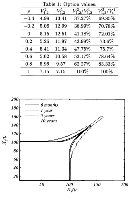
Figure 2 illustrates the investment boundaries $\partial S_{1,2}^{2}(t),$ $6$ months, 1 year, 5 years, and 10 years before maturity. The investment boundary is composed of two parts (a) and (b) with a

vertex on $(x_{1}^{1}(t), x_{2}^{1}(t))$ which is a pair of the investment triggers in a monopoly with a _single

project.11

Needless to say, the investment region becomes larger as time to maturity. This

implies that the option value increases with time to maturity. In fact, the option values 6

months, 1 year, 5 years, and 10 years before maturity are $V_{1,2}^{2}=$ 3.72,5.15,9.83, and 12.16, respectively.

Let us

now

examine the effects of the correlation coefficient $\rho$, which is the most interesting

feature in the model. Fix time to maturity as 1 year. Figure 3 depicts the investment boundary $\partial S_{1,2}^{2}(t)$ in aduopoly with those of

a

monopoly with twoprojects, i.e.,

$\partial S_{1,2}^{1}(t)$. The investment

boundary in a duopoly, unlike that of a monopoly, is independent of the correlation. We

see

from Figure 3 that the investment region in a monopoly becomes smaller with the correlation. In other words, the monopolistic option value decreases with the diversification effects.

Table 1 presents the option values and percentages for a range of correlation coefficients $\rho$.

The option value$V_{1,2}^{2}$ in aduopoly increases to _{$V_{i}^{1}=7.15$} with

$\rho$, while the option value$V_{1,2}^{1}$ in a

monopoly drops to $V_{i}^{1}=7.15$,

as

shown in the previous subsection. For

a

_{reasonable correlation}

$\rho=-0.2\sim 0.8$ the option value inaduopoly is 40% $\sim$ 60% of the monopolist withtwo projects,

or equivalently 70% $\sim$ 80% of the monopolist with asingle project.

It should be noted that the results concerning the percentages $V_{1,2}^{2}/V_{1,2}^{1},$$V_{1,2}^{2}/V_{i}^{1}$ are robust for time to maturity $T$, drift

$\mu$, and volatility $\sigma$

.

For example, for $\rho=0$, the option value

10 years before maturity is $V_{1,2}^{2}=12.16$, which is more than twice that of Table 1, while the

percentages are $V_{1,2}^{2}/V_{1,2}^{1}=$

42.72%,

$V_{1,2}^{2}/V_{i}^{1}=$ 74.73%. The option value and the percentages

for volatility $\sigma=0.5$ _{and $\rho=0$} are _{$V_{1,2}^{2}=12.32$ and} $V_{1,2}^{2}/V_{1,2}^{1}=$

38.87%,

$V_{1,2}^{2}/V_{i}^{1}=$

69.99%,

respectively.

Inavaluation ofaproject byarealoptions approach, itsometimes

occurs

that amonopolistic model and strategic model generate polar valuations, namely, the value in the former istoohigh 1lAllcomputationsin thepaper useabivariate version of the lattice binomial method with500time steps, and

while that in the latter becomes too low. Then, a substantial problem for a practitioner arises. How can we judge the gap and which value is reliable? The model of the paper would provide

us with a useful criterion in such a case. That is, we should evaluate the value of a project considering a potential alternative using the methodology of this paper.

Table 1: Option values.

$\frac{\rho V_{1,2}^{2}V_{1,2}^{1}V_{12}^{2}/V_{12}^{1}V_{12}^{2}/V_{i}^{1}}{-0.44.9913.4137.27\% 69.85\%}$ $-0.2$

5.06

12.99

38.99% 70.78% $0$ 5.15 12.51 41.18% 72.01% 0.2 5.26 11.97 43.99% 73.6% 0.4 5.41 11.34 47.75% 75.7% 0.6 5.62 10.58 53.17% 78.64% 0.8 5.96 9.57 62.27% 83.33% 1 7.15 7.15 100% 100%

Figure 2: The preemptive boundary $\partial S_{1,2}^{2}(t),$ $0.5,1,5$, and 10 years before maturity.

4

Conclusion

This paper has investigated the preemptive equilibrium in a real options model with the mul-tidimensional state variable, which represents potential alternative projects. The results

are

Figure 3: The investment boundary $\partial S_{1,2}^{2}(t)$ and $\partial S_{1,2}^{1}(t)$ for $\rho=0,0.4$, and 0.8.

First, preemptive investment takes place earlier and the option value becomes lower if the numbers of both firms and projectsincrease by the same amount. The result can be regarded as

extension of the previousresultswith a one-dimensional state variable aswell

as

being consistent with empirical findings.

Second, _{the preemptive competition is moderated by the correlation among profits from}

projects. The effect contrasts withthat in a monopoly where astrong correlation decreases the value of project _{choice. The sensitivity of the correlation to the project value in an oligopoly} depends on atrade-offbetween moderation of thepreemptive competition and a decrease in the value of project choice.

Third, the strategic option values with a symmetricalternative is 40% $\sim$60% ofa monopoly

with two alternative projects, or equivalently 70% $\sim$ 80% of

a

monopoly with

a

single project.

This indicatesthe importanceof the existence ofapotential alternative. Althoughmonopolistic

and strategic modelswith

_{a one-dimensional}

_{statevariable tend to calculate extreme values, the} method in this paper allows a reasonable valuation taking account of the follower’s potential

alternative investment.

Lastly, I should point _{out important but difficult topics for future research. The paper}

assumes

that profits from the projects

are

not sensitive to acompetitor’s _{altemative investment.}

However, the leader’s cash flow could be affected by the follower’s initiation of a project

even

if it is an altemative project that is different _{from the leader’s project. Also, the projects may}

References

[1] A. F. Azevedo and D. A. Paxson. New technology adoption games: An application to the textile industry. Real Options Conference, Rio de Janeiro, 2008.

[2] J. D\’ecamps, T. Mariotti, and S. Villeneuve. Irreversible investment in alternative projects. Economic Theory, 28:425-448, 2006.

[3] J. Detemple. American-Style Derivatives valuation and computation. Chapman

&

$Hal1/$CRC, London, 2006.

[4] A. Dixit and R. Pindyck. Investment Under Uncertainty. Princeton University Press, Princeton, 1994.

[5] D. Geltner, T. Riddiough, and S. Stojanovic. Insights

on

the effect of land

use

choice: The perpetual option on the best of two underlying assets. Joumal

_of

Urban Economics, 39:20-50, 1996.

[6] S. Grenadier. The strategic exercise ofoptions: development cascades and overbuilding in

real estate markets. Joumal

_of

Finance, 51:1653-1679, 1996.

[7] S. Grenadier. Optionexercisegames:

an

application tothe equilibrium investment strategies of firms. Review

_of

Financial Studies, 15:691-721, 2002.

[8] S. Grenadier and N. Wang. Investment timing, agency, and information. Joumal

_of

Finan-cial Economics, 75:493-533, 2005.

[9] K. Huisman. Technology Investment: A Game Theoretic Real Options Approach. Kluwer Academic Publishers, Boston, 2001.

[10] J. Jou and T. Lee. Irreversible investment financing and bankruptcy decisions in an

oligopoly. Joumal

_of

Financial and Quantitative Analysis, 43:769-786, 2008.

[11] H. Louberg\’e,

S.

Villeneuve, and M. Chesney. Long-term risk management of nuclear waste:

a real options approach. Joumal

_of

Economic Dynamics and Control, 27:157-180, 2002.

[12] M. Nishihara. Preemptive investment game with alternative projects. Discussion Papersin Economics and Business, Osaka University 09-16, 2009.

[13] M. Nishihara. Hybrid or electric vehicles? a real options perspective. Opemtions Research Letters, forthcoming, 2010.

[14] M. Nishihara and A. Ohyama. R&D competitionin alternative technologies: A real options approach. Journal

_of

the Operations Research Society

_of

Japan, 51:55-80, 2008.

[15] E. Schwartz and W. Torous. Commercial office space: Testing the implications of real

[16] T. Shibata and M. Nishihara. Dynamic investment and capital structure under

manager-shareholder conflict. Journal

_of

Economic Dynamics and Control, 34:158-178, 2010. [17] H. Weeds. Strategic delayin areal options modelof

r&d

competition. Review

_of

Economic

Studies, 69:729-747, 2002.

[18] A. Zhdanov. Competitive equilibrium with debt. Joumal

_of

Financial and Quantitative