短パルスモデル方程式の周期解
Periodic solutions of
the short pulse
model equation
山口大学大学院理工学研究科
松野
好雅
(Yoshimasa Matsuno)
Division of
Applied
Mathematical
Science
Graduate
School of
Science
and Engineering
Yamaguchi University
Abstract
The short
pulse model
equation
describes
the
propagation
of
ultra-short
optical
pulses
in nonlinear media. We
develop
a
systematic
method for solving the short
pulse equation
and address the construction of the
two-phase periodic
solutions
and
their properties.
The detail
of the content
of this paper is
described in Ref.
[11].
1.1 Maxwell equation
We
start from
the following Maxwell equation
$divD=\rho$
,
$divB=0$
,
rot
$E=-\frac{\partial B}{\partial t}$,
rot
$H=j+\frac{\partial D}{\partial t}$(l.la)
$D=\epsilon_{0}E+P$
,
$B=\mu_{0}H$
$($1.1
$b)$where
$E$
and
$H$
are
electric and magnetic field vectors,
respectively,
and
$D$
and
$B$
are
corresponding
electric and
magnetic
flux
density.
We
assume
that
$\rho=0$
and
$j=0$
and consider the
one-dimensional
propagation.
Then
Eq.
(1.1)
reduces
to
$E=E_{3}(x, t)e_{3}$
,
$H=H_{2}(x, t)e_{2}$
(1.2)
$\frac{\partial H_{2}}{\partial x}=\frac{\partial D_{3}}{\partial t}$
,
$\frac{\partial E_{3}}{\partial x}=\mu_{0}\frac{\partial H_{2}}{\partial t}$.
(1.3)
Using
(1.3)
and the relation
$D_{3}=\epsilon_{0}E_{3}+P_{3}$
,
we
eliminate
$H_{2}$from
(1.3) to
obtain
$E_{xx}- \frac{1}{c^{2}}E_{tt}=P_{tt}$
(14)
where
we
have
put
$E=E_{3},$
$P=P_{3}/(\epsilon_{0}c^{2}),$
$c^{2}=(\epsilon_{0}\mu_{0})^{-1}$.
We further
assume
the
relation
$P=P_{lin}+P_{nl}= \int_{-\infty}^{\infty}\chi(t-\tau)E(x, \tau)d\tau+\chi_{3}E^{3}$
$(1.5a)$
Substituting
(1.5)
into
(1.4),
we
obatin the nonlinear
wave
equation
$E_{xx}- \frac{1}{c^{2}}E_{tt}=\chi_{0}E+\chi_{3}(E^{3})_{tt}$
.
(1.6)
1.2 Singular
perturbation
In accordance with
Sch\"afer
and Wayne (2004),
we
apply
the
singular
perturba-tion
method
to Eq. (1.6) to
derive the short
pulse (SP) equation.
We
expand
$E$
with
respect
to the small
parameter
$\epsilon$$E(x, t)=\epsilon u_{0}(\phi, X)+\epsilon^{2}u_{1}(\phi, X)+\cdots$
$(1.7a)$
where
the
new
independent
variables
$\phi$and
$X$
are
defined
by
$\phi=\frac{t-\frac{x}{c}}{\epsilon}$
,
$X=\epsilon x$
.
$(1.7b)$
If
we
introduce
(1.7)
into
(1.6),
we
obtain, at
the lowest order
$O(\epsilon)$,
the
following
PDE
$- \frac{2}{c}\frac{\partial^{2}u_{0}}{\partial\phi\partial X}=\chi_{0}u_{0}+\chi_{3}\frac{\partial^{2}u_{0}^{3}}{\partial\phi^{2}}$
.
(1.8)
After
an
appropriate change
of the
variables,
we
arrive at
the normalized form of
the
SP
equation:
$u_{xt}=u+ \frac{1}{6}(u^{3})_{xx}$
.
(1.9)
1.3 Remarks
$\bullet$
The
SP
equation
is
a
model
equation
describing
the
propagation
of
ultra-short
optical pulses
in nonlinear media.
$\bullet$
The
SP
equation
has been derived
in
a
mathematical context conceming the
integrable
PDE
(Robelo (1989)).
$\bullet$
The
following solutions
are
known
for the
SP
equation:
Soliton
and
breather
solutions:
Sakovich
et
al
(2006),
Kuetche et al
(2006),
Matsuno
(2007)
Periodic solutions of traveling
type (one-phase solutions):
Parkes
(2008)
$\bullet$
Analogous
integrable equations (Matsuno (2006))
$u_{xt}= \alpha u+\frac{1}{2}(1-\beta)u_{x}^{2}-uu_{xx}$
$\beta=2$
:
Short-pulse
model for
Camassa-Holm
equation
$\beta=3$
:
Short-pulse model
for
the Degasperis-Procesi
equation,
Vakhnenko
equa-tion
$\alpha=0,$
$\beta=2$
:
Hunter-Saxton
equation
All
the
above
equations
have the solutions
expressed
by
the
parametric
2. Exact method of solution
2.1 Transformation to the sine-Gordon
equation
Introduce
the
new
variable
$r$:
$r^{2}=1+u_{x}^{2}$
.
(2.1)
We
rewrite
the
SP
equation
(1.9)
into the
form
$r_{t}=( \frac{1}{2}u^{2}r)_{x}$
.
(2.2)
By
means
of
the
hodograph
transformation
$(x, t)arrow(y, \tau)$
$dy=rdx+ \frac{1}{2}u^{2}rdt$
,
$d\tau=dt$
$(2.3a)$
or
equivalently
$\frac{\partial}{\partial x}=r\frac{\partial}{\partial y},$ $\frac{\partial}{\partial t}=\frac{\partial}{\partial\tau}+\frac{1}{2}u^{2}r\frac{\partial}{\partial y}$
$(2.3b)$
(2.1)
and
(2.2)
are
transformed
to
$r^{2}=1+r^{2}u_{y}^{2}$
,
$r_{\tau}=r^{2}uu_{y}$
.
(2.4)
Using
the
transformation
$u_{y}=\sin\phi$
,
$\phi=\phi(y, \tau)$
(2.5)
(2.4)
can
be
put
into
the form
$\frac{1}{r}=\cos\phi$
.
(2.6)
It
follows from
$(2.4)-(2.6)$
that
$u=\phi_{\tau}$.
Substituting this into
(2.5),
we
obtain the
sine-Gordon
$(sG)$
equation
:
$\phi_{y\tau}=\sin\phi$
.
(2.7)
We
see
from
(2.3)
that
$x=x(y, \tau)$
satisfies
the
following linear PDE
$x_{y}= \frac{1}{r}$
,
$x_{\tau}=- \frac{1}{2}u^{2}$.
(2.8)
2.2
Parametric
representation of the solution
Since
the
integrability of
Eq.
(2.8), i.e.
$x_{y\tau}=x_{\tau y}$is
assured by
(2.4),
we
can
integrate (2.8)
to
obtain
$x(y, \tau)=\int^{y}\cos\phi dy+d$
(2.9)
where
$d$is
an integration
constant.
The
expression
of
$u$in
terms
$\phi$is
given by
2.3 A
criterion
for the
single-valued functions
To derive
a
criterion for
single-valued functions,
we
may
simply require
that
$u_{x}=\tan\phi$
exhibits
no
singularities. Thus,
if
$- \frac{\pi}{2}<\phi<\frac{\pi}{2}$
,
$(mod \pi),$
$(- \sqrt{2}+1<\tan\frac{\phi}{4}<\sqrt{2}-1)$
.
(2.11)
then the
parametric
solutions
(2.9) and (2.10) will
become
single-valued
functions
for
all values
of
$x$and
$t$.
3. Periodic solutions
Here,
we are
concemed
with the construction of
the
periodic
solutions of the
SP
equation, particularly
focusing
on
the
two-phase
solutions.
3.1
Method
of solution
We first introduce the
two independent phase
variables
$\xi$and
$\eta$according
to
$\xi=ay+\frac{t}{a}+\xi_{0},$
$\eta=ay-\frac{t}{a}+\eta_{0}$
(3.1)
where
$a(\neq 0),$
$\xi_{0}$and
$\eta_{0}$
are
arbitrary constants.
Then,
the
$sG$
equation
is
trans-formed
to
$\phi_{\xi\xi}-\phi_{\eta\eta}=\sin\phi,$
$\phi=\phi(\xi, \eta)$
.
(3.2)
We seek
solutions
of
the
$sG$
equation
of the form
$\phi=4\tan^{-1}[\frac{f(\xi)}{g(\eta)}]$
.
(3.3)
This
$\phi$satisfies
the
$sG$
equation provided
that
$f^{\prime 2}=-\kappa f^{4}+\mu f^{2}+\nu$
$(3.4a)$
$g^{\prime 2}=\kappa g^{4}+(\mu-1)g^{2}-\nu$
.
$(3.4b)$
Now,
the
parametric
representation
of
$u$follows
from
(2.10)
and
(3.3)
$u= \frac{4}{a}\frac{f’g+fg^{f}}{f^{2}+g^{2}}$
.
(3.5)
To obtain the
parametric
form of
$x$,
we
note the
relation
$\cos\phi=1-\frac{8f^{2}g^{2}}{(f^{2}+g^{2})^{2}}$
.
(3.6)
We
modify
the
right-hand
side of
(3.6) by introducing
the
function
$Y=Y(\xi, \eta)$
We calculate
$Y_{y}$.
Using (3.4),
we can
modify
this in the form
$Y_{y}= \frac{a}{(f^{2}+g^{2})^{2}}[-2\kappa(c_{1}f^{6}+3c_{1}f^{4}g^{2}-3c_{2}f^{2}g^{4}-c_{2}g^{6})-4c_{2}f^{2}g^{2}$
$+2(c_{1}+c_{2})\{-2fgf’g’+2\mu f^{2}g^{2}-\nu(f^{2}-g^{2})\}]$
.
(3.8)
If
we
put
$c_{1}+c_{2}=0$
and
$c_{1}=-2/a$
,
then
(3.8)
simplifies
to
$Y_{y}=4 \kappa(f^{2}+g^{2})-\frac{8f^{2}g^{2}}{(f^{2}+g^{2})^{2}}$
.
(3.9)
If
we
compare
(3.6)
and
(3.9),
we
obtain
$\cos\phi=1+Y_{y}-4\kappa(f^{2}+g^{2})$
.
(3.10)
Finally,
substituting (3.10) into (2.9) and
integrating,
we
obtain the
parametric
representation
of
$x$:
$x=y- \frac{4}{a}\frac{ff’-gg’}{f^{2}+g^{2}}-\frac{4\kappa}{a}(\int f^{2}(\xi)d\xi+\int g^{2}(\eta)d\eta)+d$
.
(3.11)
3.2
Examples
Here,
we
present
the
three
examples of the periodic
solutions:
$a$.
Example 1
$f(\xi)=A$
cn
$(\beta\xi, k_{f}),$ $g( \eta)=\frac{1}{cn(\Omega\eta,k_{g})}$(312)
$k_{f}^{2}= \frac{A^{2}}{1+A^{2}}(1+\frac{1}{\beta^{2}(1+A^{2})})$
$(3.13a)$
$k_{g}^{2}= \frac{A^{2}}{1+A^{2}}(1-\frac{1}{\Omega^{2}(1+A^{2})})$
$(3.13b)$
$\Omega^{2}=\beta^{2}+\frac{1-A^{2}}{1+A^{2}}$
.
$(3.13c)$
The inequality
$0\leq k_{f}\leq 1$
implies
that
the parameter
$\beta$must
be
restricted
by
the
condition
$\frac{A}{\sqrt{1+A^{2}}}\leq\beta$
.
(3.14)
The
parametric
solution takes the form
$u= \frac{4A}{a}\frac{-\beta sn(\beta\xi,k_{f})dn(\beta\xi,k_{f})cn(\Omega\eta,k_{g})+\Omega cn(\beta\xi,k_{f})sn(\Omega\eta,k_{g})dn(\Omega\eta,k_{g})}{A^{2}cn^{2}(\beta\xi,k_{f})cn^{2}(\Omega\eta,k_{g})+1}$
$(3.15a)$
$- \frac{\beta k_{f}^{2}}{\Omega k_{g}^{\prime 2}}$
cn
$(\beta\xi, k_{f})$sn
$(\Omega\eta, k_{9})$dn
$(\Omega\eta, k_{g})\}$$- \frac{4\beta}{a}[E(\beta\xi, k_{f})-k_{f}^{\prime 2}\beta\xi-\frac{\beta k_{f}^{2}}{A^{2}\Omega k_{g}^{\prime 2}}\{E(\Omega\eta, k_{g})-k_{g}^{\prime 2}\Omega\eta\}]+d$
.
$(3.15b)$
Properties of the solution
$\bullet$
The
solution
is
a
multiply peridic
function. It becomes
a
single-valued
function
if
$0<A<\sqrt{2}-1$
.
$\bullet$Under the condition
$L=m_{\xi}L_{\xi}/a=m_{\eta}L_{\eta}/a,$ $(m_{\xi}, m_{\eta})=1$
where
$L_{\xi}\equiv 4K(k_{f})/\beta$
and
$L_{\eta}\equiv 4K(k_{9})/\Omega$
,
the solution has
a
period
$\Lambda$$\Lambda=L[1-4\beta^{2}\{\frac{E(k_{f})}{K(k_{f})}-\frac{k_{f}^{2}E(k_{g})}{A^{2}(1-k_{g}^{2})K(k_{g})}+\frac{1}{\beta^{2}(1+A^{2})}\}]$
(3.16)
where
$K(k_{f})$
and
$E(k_{f})$
are
the
complete
elliptic integral of the
first
and
second
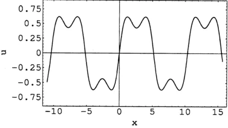
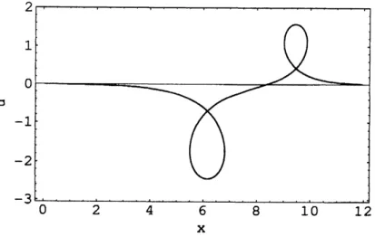
kinds, respectively. Figure 1 shows
a
profile of
$u$at
$t=0$
for Example 1.
X
Figure 1:
$A=0.2,$
$m_{\xi}=1,$ $m_{\eta}=2,$
$a=1.0,$
$\beta=0.5832,$
$\Omega=1.124,$
$k_{f}=$
0.3837,
$k_{g}=0.0958,$
$\Lambda=10.37$
.
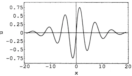
Long-wave
limit
$\Lambdaarrow\infty$In the long-wave
limit,
the
parametric
solution reduces
to
$u \sim\frac{4A\Omega}{a}\frac{-A\sinh\beta\xi\cos\Omega\eta+\cosh\beta\xi\sin\Omega\eta}{\cosh^{2}\beta\xi+A^{2}\cos^{2}\Omega\eta}$
$(3.17a)$
X
Figure 2: Long-wave limit of the solution
depicted
in Figure 1.
$b$
.
Example
2
$f( \xi)=A\frac{sn(\beta\xi,k_{f})}{cn(\beta\xi,k_{f})},$ $g( \eta)=\frac{1}{dn(\Omega\eta,k_{g})}$
(3.18)
$k_{f}^{2}=1-A^{2}+ \frac{A^{2}}{\beta^{2}(1-A^{2})}$
$(3.19a)$
$k_{g}^{2}=1- \frac{1}{A^{2}}+\frac{1}{\Omega^{2}(1-A^{2})}$
$(3.19b)$
$\Omega=\beta A$
$(3.19c)$
$\frac{1}{\sqrt{1-A^{2}}}\leq\beta\leq\frac{1}{1-A^{2}}$
(3.20)
$u= \frac{4A}{a}\frac{\beta dn(\beta\xi,k_{f})dn(\Omega\eta,k_{g})+k_{g}^{2}\Omega sn(\beta\xi,k_{f})cn(\beta\xi,k_{f})sn(\Omega\eta,k_{g})cn(\Omega\eta,k_{g})}{A^{2}sn^{2}(\beta\xi,k_{f})dn^{2}(\Omega\eta,k_{g})+cn^{2}(\beta\xi,k_{f})}$
$(3.21a)$
$x=y- \frac{4\beta}{a}\frac{1}{A^{2}sn^{2}(\beta\xi,k_{f})dn^{2}(\Omega\eta,k_{g})+cn^{2}(\beta\xi,k_{f})}\cross$
$\cross[(A^{2}dn2(\Omega\eta, k_{9})-1)$
sn
$(\beta\xi, k_{f})$cn
$(\beta\xi, k_{f})$dn
$(\beta\xi, k_{f})$$+k_{9}^{2}A^{3}$
sn2
$(\beta\xi, k_{f})$sn
$(\Omega\eta, k_{g})$cn
$(\Omega\eta, k_{g})$dn
$( \Omega\eta, k_{g})]+\frac{4\beta}{a}(-E(\beta\xi, k_{f})+AE(\Omega\eta, k_{g}))+d$
$($
3.21
$b)$$A=L[1-4\beta^{2}\{\frac{E(k_{f})}{K(k_{f})}-A^{2}\frac{E(k_{g})}{K(k_{g})}\}]$
.
(3.22)
X
Figure 3:
$A=0.2,$
$m_{\xi}=2,$ $m_{\eta}=1,$
$a=1.0,$
$\beta=1.027,$ $\Omega=0.2053,$
$k_{f}=$
0.9998,
$k_{g}=0.8421,$
$\Lambda=5.938$
.
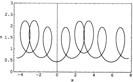
Long-wave limit
$\Lambdaarrow\infty$$u \sim\frac{4\beta A}{a}\frac{\cosh\beta\xi\cosh\Omega\eta+A\sinh\beta\xi\sinh\Omega\eta}{A^{2}\sinh^{2}\beta\xi+\cosh^{2}\Omega\eta}$
$(3.23a)$
$x \sim y-\frac{2\beta}{a}\frac{A^{2}\sinh 2\beta\xi-A\sinh 2\Omega\eta}{A^{2}\sinh^{2}\beta\xi+\cosh^{2}\Omega\eta}+d$
.
$(3.23b)$
X
Figure 4:
Long-wave limit
of the
solution
depicted
in
Figure
3.
$c$
.
Example 3
$f(\xi)=Adn(\beta\xi, k_{f}),$
$g( \eta)=\frac{cn(\Omega\eta,k_{g})}{sn(\Omega\eta,k_{g})}$(3.24)
$k_{g}^{2}=1-A^{2}+ \frac{A^{2}}{\Omega^{2}(A^{2}-1)}$
$(3.25b)$
$\Omega=\frac{\beta}{A}$
$(3.25c)$
$\frac{A}{\sqrt{A^{2}-1}}\leq\beta\leq\frac{A^{2}}{A^{2}-1},$
$A>1$
(3.26)
$u=- \frac{4A}{a}\frac{\Omega dn(\beta\xi,k_{f})dn(\Omega\eta,k_{g})+\beta k_{f}^{2}sn(\beta\xi,k_{f})cn(\beta\xi,k_{f})sn(\Omega\eta,k_{g})cn(\Omega\eta,k_{g})}{A^{2}dn^{2}(\beta\xi,k_{f})sn^{2}(\Omega\eta,k_{g})+cn^{2}(\Omega\eta,k_{g})}$
$(3.27a)$
$x=y- \frac{4\beta}{a}\frac{1}{A^{2}dn^{2}(\beta\xi,k_{f})sn^{2}(\Omega\eta,k_{g})+cn^{2}(\Omega\eta,k_{g})}\cross$
$\cross[\frac{1}{A}(1-A^{2}dn2(\beta\xi, k_{f}))$
sn
$(\Omega\eta, k_{g})$cn
$(\Omega\eta, k_{g})$dn
$(\Omega\eta, k_{g})$$-k_{f}^{2}A^{2}$
sn
$(\beta\xi, k_{f})$cn
$(\beta\xi, k_{f})$dn
$(\beta\xi, k_{f})$sn2
$( \Omega\eta, k_{g})]-\frac{4\beta}{a}(E(\beta\xi, k_{f})-\frac{1}{A}E(\Omega\eta, k_{g}))+d$
$(3.27b)$
$\Lambda=L[1-4\beta^{2}\{\frac{E(k_{f})}{K(k_{f})}-\frac{1}{A^{2}}\frac{E(k_{g})}{K(k_{g})}\}]$
.
(3.28)
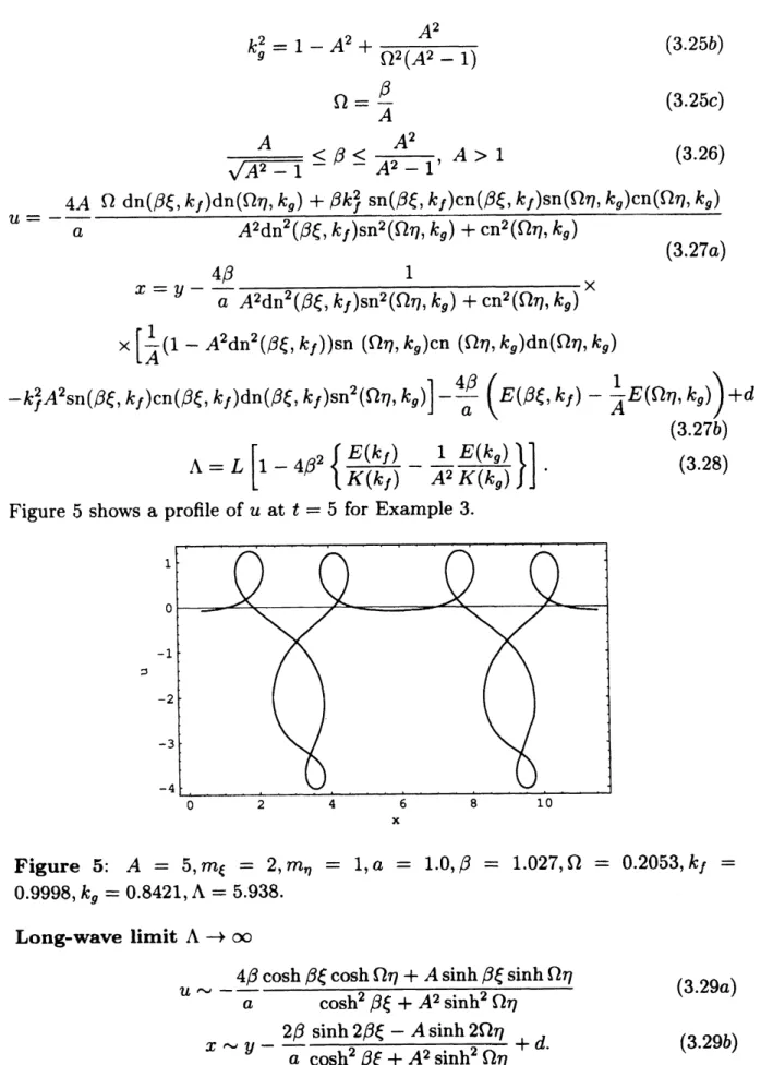
Figure
5
shows
a
profile of
$u$at
$t=5$
for
Example
3.
$x$
Figure 5: $A=5,$
$m_{\xi}=2,$
$m_{\eta}=1,$
$a=1.0,$
$\beta=1.027,$ $\Omega=0.2053,$
$k_{f}=$
0.9998,
$k_{g}=0.8421,$
$\Lambda=5.938$
.
Long-wave
limit
$\Lambdaarrow\infty$$u \sim-\frac{4\beta}{a}\frac{\cosh\beta\xi\cosh\Omega\eta+A\sinh\beta\xi\sinh\Omega\eta}{\cosh^{2}\beta\xi+A^{2}\sinh^{2}\Omega\eta}$
$(3.29a)$
X
Figure
6:
Long-wave limit of the solution
depicted
in Figure
5.
4.
Conclusion
$\bullet$
By
means
of
a
novel
method
of exact solution,
we
obtained
periodic
solutions
of
the
SP
equation
and investigated
their
properties.
$\bullet$
Of
particular
interest is the nonsingular
periodic
solution which reduces
to
the
breather solution
in
the
long-wave
limit.
$\bullet$