An equality test of high-dimensional covariance matrices under the SSE model (Statistical Inference and Modelling)

全文

(1)22. An equality test of high‐dimensional covariance matrices under the SSE model Kazuyoshi Yata Institute of Mathematics. University of Tsukuba Aki Ishii. Department of Information Sciences Tokyo University of Science Makoto Aoshima. Institute of Mathematics. University of Tsukuba. Abstract. In this paper, we consider an equality test of high‐dimensional covariance matrices under the strongly spiked eigenvalue (SSE) model. We introduce an eigenvalue model called the “strongly spiked eigenvalue (SSE) model” which was proposed by Aoshima and Yata (2018). We give a new test procedure based on the spiked eigenstructures.. 1. Introduction. Suppose we have two classes. \pi_{i},. i=1,2 . We define independent d\cross n_{i} data matrices,. n_{i} , are independent and X_{i}=[x_{i1}, x_{in_{\iota}}], i=1,2 , for \pi_{i}, i=1,2 , where x_{ij}, j=1, identically distributed (i.i. d. ) as a d‐dimensional distribution with a mean vector \mu_{i} and covariance matrix \Sigma_{i}(\geq O) . We assume n_{i}\geq 4, i=1,2 . The eigen‐decomposition of \Sigma_{i}. is given by. \Sigma_{i}=H_{i}A_{i}H_{i}^{T},. where A_{i}=diag(\lambda_{1(i)}, \ldots, \lambda_{d(i)}) having \lambda ı(i). \geq. \geq\lambda_{d(i)}(\geq 0) and. an orthogonal matrix of the corresponding eigenvectors. Let. X_{i}-[\mu_{i}, \mu_{i}]=H_{i}A_{i}^{1/2}Z_{i}. H_{i}=. [hı(i),. h_{d(i)} ] is.

(2) 23 for i=1,2 . Then, Z_{i} is a d\cross n_{i} sphered data matrix from a distribution with the zero mean and identity covariance matrix. Let. Z_{i}=[z_{1(i)}, z_{d(i)}]^{T}. z_{j(i)}=(z_{j1(i)}, \ldots, z_{jn_{x}(i)})^{T},. and. j=1,. d. for i=1,2 . Note that E(z_{jk(i)}z_{j'k(i)})=0(j\neq j') and Var(z_{j(i)})=I_{n_{\iota}} , where I_{n}, denotes the n_{i} ‐dimensional identity matrix. Also, note that if X_{i} is Gaussian, z_{jk(i)}s are i.i. d . as the standard normal distribution, N(0,1) . We assume that the fourth moments of each variable in Z_{i} are uniformly bounded for i=1,2 . Also, we consider the following assumption:. (A‐i). E(z_{qj(i)}^{2}z_{sj(i)}^{2})=1. and E(z_{qj(i)}z_{sj(i)}z_{tj(i)}z_{uj(i)})=0 for all q\neq s, t, u. This kind of assumption was made by Bai and Saranadasa (1996), Chen and Qin (2010) and Aoshima and Yata (2011). We note that (A‐i) naturally holds when X_{i} is Gaussian. We consider a test problem as follows:. vs.. H_{0}:\Sigma_{1}=\Sigma_{2}. H_{1}:\Sigma_{1}\neq\Sigma_{2} .. (1). Schott (2007) gave a test procedure when d/n_{i}arrow c_{i}\in[0, \infty ) and normal distribution. Aoshima and Yata (2011) gave a test procedure based on the quantity of tr(\Sigma_{1}-\Sigma_{2}) . They also discussed sample size determination so as to have prespecified size and power simultaneously. Li and Chen (2012) and Endo et al. (2018) considered the test problem by using the quantity of tr\{(\Sigma_{{\imath} -\Sigma_{2})^{2}\} . The above literatures discussed asymptotic properties of their test procedures when darrow\infty and n_{i}arrow\infty under the following eigenvalue condition:. \frac{\lambda_{1(i)}^{2}{tr(\Sigma_{\dot{i}^{2})arow0. as. darrow\infty. for i=1,2 .. (2). Aoshima and Yata (2018) called (2) the “non‐strongly spiked eigenvalue (NSSE) model” On the other hand, Ishii et al. (2016) investigated asymptotic properties of the first principal component and considered the test problem (1) when darrow\infty while n_{i}s are fixed under the following eigenvalue condition:. \lim_{dar ow}\inf_{\infty}\{ frac{\lambda_{1(\dot{\iota})^{2}{tr(\Sigma_{i}^ {2})\}>0. for. i=1. or 2.. (3). Aoshima and Yata (2018) called (3) the “strongly spiked eigenvalue (SSE) model” and showed that high‐dimensional data often have the SSE model. Ishii (2017a, b) considered two‐sample tests under the SSE model when darrow\infty while. n_{i}s. are fixed. The SSE model. is very difficult to handle because of the influence of strongly spiked noise. Aoshima and Yata (2018) created a data‐transformation technique for twosample tests which transforms the SSE model to the NSSE model. In this paper, we focus on the SSE model and give a new test procedure for (1) by using a different approach from the data‐transformation technique.. In Section 2, we introduce the test statistic given by Li and Chen (2012). We em‐ phasize that one should construct test procedures by considering the eigenstructure of high‐dimensional data. In Section 3, we give a new test procedure under the SSE model..

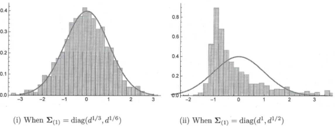
(3) 24 2. Performance of the earlier test procedure under the SSE model. In this section, we investigate the performance of the test procedure given by Li and Chen (2012). For (1) they assumed. tr(\Sigma_{i}\Sigma_{j}\Sigma_{k}\Sigma_{l})=0\{tr(\Sigma_{i}\Sigma_{j}) tr(\Sigma_{k}\Sigma_{l})\} for any i, j,. k. (4). and l\in\{1,2\} . Note that (4) is one of the NSSE models. They proposed a. test statistic as follows:. U=A_{n_{1}}+A_{n_{2}}-2tr(S_{1n_{1}}S_{2n_{2}}) ,. (5). where S_{in_{\iota} is the sample covariance matrix having E(S_{in_{z}})=\Sigma_{i} and. A_{n_{i} = \frac{1}{n_{i}(n_{\dot{i} -1)}\sum_{j\neq k}^{n_{l} (X_{ij kjl} ^{\tau_{x_{ik})^{2}-\frac{2}{n_{i}(n_{i}-1)(n_{i}-2)}\sum_{j\neq k\neq\iota}^{n_ {i} x^{T}x_{i}x_{ij}^{T}x_{\dot{i} } + \frac{1}{n_{i}(n_{i}-1)(n_{i}-2)(n_{\dot{i} -3)}\sum_{j\neq k\neq l\neq l'} ^{n_{l} x_{ij}^{T}x_{ik}x_{il}^{T}x_{il'}. Note that U is an unbiased estimator of. | \Sigma_{1}-\Sigma_{2}||_{F}^{2}=tr\{(\Sigma_{1}-\Sigma_{2})^{2}\} ( =\triangle , say). In this paper, we consider the divergence condition such as darrow\infty, which is equivalent to marrow\infty. ,. n_{1}arrow\infty. and. n_{2}arrow\infty,. where m= \min\{d, n_{1}, n_{2}\}.. Under (4) and some regularity conditions, they showed the following asymptotic result:. \frac{U-\Delta}{Var(U)^{1/2} \Rightar ow N(0,1) a Here,. "\Rightarrow. s. marrow\infty. .. (6). denotes the convergence in distribution and N(0,1) denotes a random variable. distributed as the standard normaı distribution.. Let us show a toy example about the asymptotic null distribution of U in (6). We set n2 =100 . We assumed N_{d}(0, \Sigma) for each class under H_{0}:\Sigma_{1}=\Sigma_{2}= \Sigma . Let us write a k\cross l zero matrix by O_{k,l} . We set d=2048 and nı. =. \Sigma=. (o_{d-2,2}^{\Sigma}(1) O_{2,d-2 ,\Sigma_{(2)} ). having. \Sigma_{(2)}=(0.3^{|i-j|}). and considered two cases:. (i). \Sigma_{(1)}=diag(d^{1/3}, d^{1/6}). and. (ii). \Sigma_{(1)}=diag(d^{1}, d^{1/2}) ..

(4) 25. (i) When \Sigma_{(1)}=diag(d^{1\int 3}, d^{1/6}). (ii) When \Sigma_{(1)}=diag(d^{1}, d^{1/2}). Figure 1: The histograms of (normalized) U for a NSSE model (in the left panel) and for a SSE model (in the right panel). The solid line denotes the p.d. f. of N(0,1) . Note that (i) is a NSSE model and (ii) is a SSE model. We generated independent pseudo‐ random observations from each class and calculated (normalized) U 1000 times. In Fig.1, we gave histograms for (i) and (ii). One can observe that U does not converge to N(0,1) for (ii). In order to overcome this inconvenience, we modify U under a SSE model and newly construct a test procedure for the SSE model in Section 3.. 3. Modification of U under a SSE model We assume the following assumption for the eigenvaıues:. (A‐ii). \frac{\sum_{s-2}^{d}\lambda_{s(\dot{i})^{2}{\lambda_{1(i)}^{2}=o(1). as. darrow\infty. for i=1,2.. Note that (A‐ii) is one of the SSE models. Also, note that (A‐ii) implies the conditions. that \lambda_{2(i)}/\lambda_{1(i)}arrow 0 and. \lambda_{1(i)}^{2}/tr(\Sigma_{i}^{2})ar ow 1. \lambda_{j(i)}=a_{j(i)}d^{\alpha_{J(i)}}(j=1, \ldots, k_{i}). as. darrow\infty .. and. with positive (fixed) constants, a_{j(i)}s, c_{j(i)}s and (A‐ii) holds when \alpha_{1(i)}>1/2 and \alpha_{1(i)}>\alpha_{2(i)}.. For a spiked model as. \lambda_{j(i)}=c_{j(i)}(j=k_{i}+1, \ldots, d) \alpha_{j(i)}s ,. and a positive (fixed) integer k_{i},. In addition, we consider the following condition:. (. A ‐iii). For all i, j,. z_{1j(i)}, j=1,. n_{i}. , are i.i. d . as N(0,1) for i=1,2.. E\{(z_{{\imath} j(i)}^{2}-1)^{2}\}=2 under. ( A‐iii). Let. K=2\lambda_{1({\imath})}^{2}/n_{1}+2\lambda_{1(2)}^{2}/n_{2}. We have the following result..

(5) 26 Lemma 1 (Ishii et al., 2017). Under (A‐i) to ( A ‐iii) and H_{0} , it holds that as. U=( \sum_{j={\imath} ^{n_{1} \un(zd_e{1rjl(in1)e}{^\2la}-m1)b_d{-a\_s{u1m}_{k={\imath} ^{n_{2} \frac{\lambda_{1(2)}(z_{1k(2)}^{2} -1)}{n_{2} )^{2}-K}n_{1}+o_{p}(K) (ı). Let. marrow\infty. .. T=U/K+1. Then, we have an asymptotic distribution of. T. under H_{0}.. Theorem 1 (Ishii et al., 2017). Under (A‐i) to (A ‐ii i) and H_{0} , it holds that as. marrow\infty. T\Rightar ow\chi_{1}^{2}. Here, \chi_{\nu}^{2} denotes a random variable distributed as a \chi^{2} distribution with. \nu. degrees of. freedom.. Since \lambda ı(i)s are unknown, we need to estimate them. It is well known that the sample. eigenvalues get too much noise for high‐dimensional data. See Jung and Marron (2009), Yata and Aoshima (2009), Ishii et al. (2016) and Shen et al. (2016) for the details. We consider estimating \lambda ı(i)s by using the noise‐reiuction (NR) methodology given by Yata and Aoshima (2012). We denote the dual matrix of S_{in_{t}} by S_{Dn_{l}} and define its eigen‐ decomposition as follows:. S_{iD}=(n_{i}-1)^{-1}(X_{i}-\overline{X}_{i})^{T}(X_{i}-\overline{X}_{i}). =\sum_{s={\imath}^{n_{l}-1\hat{\lambda}_{s(i)}\hat{u}_{s(i)}\hat{u}_{s(i)} ^{T}, where. \overline{X}_{i}=[\overline{x}_{i}, \overline{x}_{i}]. \lambda_{j(i)}s are estimated by. and. \overline{x}_{i}=n_{i}^{-1}\sum_{j=1}^{n_{l} x_{ij}. for i=1,2 . If one uses the NR method,. \tilde{\lambda}_{j(i)}=\hat{\lambda}_{j(i)}-\frac{tr(S_{iD})-\sum_{s=1}^{j} \hat{\lambda}_{s(i)} {n_{i}-1-j} (j=1, \ldots, n_{i}-2) Note that. \tilde{\lambda}_{j(i)}\geq 0. w.p.1 for j=1,. n_{i}-2 .. that \tilde{\lambda}_{j (i) has consistency properties when. Yata and Aoshima (2012, 2013) showed. darrow\infty. and. n_{i}arrow\infty. Ishii et al. (2016) gave asymptotic properties of \tilde{\lambda}_{1} (i) when. s_{1(i)}= \sum_{j=1}^{n_{l}}(z_{{\imath} j(i)}-\overline{z}_{1(i)})^{2}/(n_{i}- 1). .. for i=1,2 , where. . On the other hand,. darrow\infty. while. \overline{z}_{1(i)}=n_{i}^{-{\imath} \sum_{j=}^{n_{l} ı. n_{i}. is fixed. Let. z_{1j(i)}.. Theorem 2 (Yata and Aoshima, 2013 and Ishii et al., 2016). Under (A‐i) and (A‐ii), holds that as darrow\infty. \frac{\tilde{\lambda}_{1(i)}{\lambda_{1(i)}=\{ begin{ar ay}{l} s{\imath}(i)+op(l) when _{i} sfixed, 1+o_{p}(1) when _{i}ar ow\infty. \end{ar ay}. it.

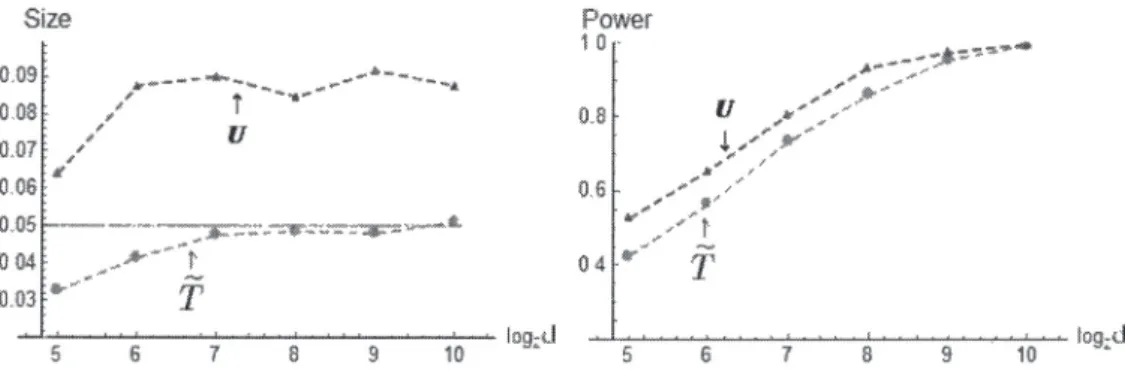
(6) 27. Under (A‐i) to ( A ‐iii), it holds that as. darrow\infty. (n_{i}-1)\frac{\overline{\lambda}_{1(i)}{\lambda_{1(i)} \Rightar ow\chi_{n_{t}-1^{2} and. when. \sqrt{\frac{n_{i}-1}{2} (\frac{\tilde{\lambda}_{1(i)} {\lambda_{1(i)} -1) \Rightar ow N(0,1). n_{i}. is fixed,. when n_{i}arrow\infty.. \tilde{K}=2\tilde{\lambda}_{ \imath}(1)}^{2}/n_{1}+2\tilde{\lambda}_{1(2)}^{2} /n_{2} and. Let. \overline{T}=U/\tilde{K}+1. We have the following result.. Theorem 3 (Ishii et al., 2017). Under (A‐i) to ( A ‐iii) and H_{0} , it holds that as. marrow\infty. \tilde{T}\Rightar ow\chi_{1}^{2}. We consider testing (1) for a given \alpha\in(0,1/2) by. rejecting where c_{1}(\alpha) denotes the upper. \alpha. H_{0}\Leftrightarrow\overline{T}\geq c_{1}(\alpha) ,. (7). point of \chi_{1}^{2} . Then, under (A‐i) to ( A ‐iii), it holds that as. marrow\infty. Size. =\alpha+o(1) .. See Ishii et al. (2017) for the asymptotic power of the test procedure by (7). 4. Simulation. We compared the performance of the test by \overline{T} with the test by U in numerical simu‐ lations. Independent pseudo‐random observations were generated from N_{d}(0, \Sigma_{i}) . We set \alpha=0.05 and. \Sigma_{i}= (0_{d-2,2}^{\Sigma_{i(1)} \Sigma_{i(2)}^{O_{2,d-2} ), i=1,2, where. O_{k,l}. is the k\cross l zero matrix. We set. \Sigma_{1(1)}=diag(d^{2/3}, d^{1/2}). and. \Sigma_{1(2)}=(0.3^{|i-j|^{i/3}}) .. As for the alternative hypothesis, we considered \Sigma_{2}=2\Sigma_{1} . Note that (A‐i) to ( A ‐iii) are d=2^{8} for s=5 , 10, where \lceil x\rceil denotes. met. We set (n_{1}, n_{2})=(\lceil 3d^{1/2}\rceil, \lceil 4d^{1/2}\rceil) and the smallest integer \geq x..

(7) 28. g\propto-d. Figure 2: The performances of the tests by \overline{T} and U . We set (n_{1}, n_{2})=(\lceil 3d^{1/2}\rceil, \lceil 4d^{1/2}\rceil) and d=2^{S} for s=5 , 10. The values of \overline{\alpha} are denoted by the dashed lines in the left panel and the vaıues of 1-\overline{\beta} are denoted by the dashed lines in the right panel.. We checked the performance by 2000 replications. We defined P_{r}=1 (or 0 ) when H_{0} was falsely rejected (or not) for r=1 , 2000, and defined \overline{\alpha}=\sum_{r=1}^{2000}P_{r}/2000 to estimate the size. We also defined P_{r}=1 (or 0 ) when H_{1} was falsely rejected (or not) for r=1 ,. 2000, and defined. 1- \overline{\beta}=1-\sum_{r=1}^{2000}P_{r}/2000. to estimate the power. Note that. their standard deviations are less than 0.011. In Fig. 2, we plotted \overline{\alpha} (left panel) and 1-\overline{\beta} (right panel). One can observe that the test by \overline{T} gave preferable performances. On the other hand, the test by. U. gave a bad performance with respect to the size. Remember that. U. was. constructed under (2). We emphasize that it is very important to select a suitable test procedure depending on the eigenstructure.. Acknowledgements Research of the first author was partially supported by Grant‐in‐Aid for Scientific Re‐. search (C), Japan Society for the Promotion of Science (JSPS), under Contract Number 18K03409 . Research of the second author was partially supported by Grants‐in‐Aid for Young Scientists, JSPS, under Contract Number 18K18015 . Research of the third au‐. thor was partially supported by Grants‐in‐Aid for Scientific Research (A) and Challenging Research (Exploratory), JSPS, under Contract Numbers 15H01678 and 17K19956..

(8) 29 References. [ı] Aoshima, M., Yata, K., 2011. Two‐stage procedures for high‐dimensional data. Se‐ quential Anal. (Editor’s special invited paper) 30, 356‐399.. [2] Aoshima, M., Yata, K., 2018. Two‐sample tests for high‐dimension, strongly spiked eigenvalue models. Stat. Sin. 28, 43‐62.. [3] Bai, Z., Saranadasa, H., 1996. Effect of high dimension: By an example of a two sample problem. Stat. Sin. 6, 311‐329.. [4] Chen, S.X., Qin, Y.‐L., 2010. A two‐sample test for high‐dimensional data with ap‐ plications to gene‐set testing. Ann. Statist. 38, 808‐835.. [5] Endo, K., Yata, K., Aoshima, M., 2018. A test for high‐dimensional covariance matri‐ ces via the extended cross‐data‐matrix methodology. RIMS Kokyuroku, submitted.. [6] Ishii, A., Yata, K., Aoshima, M., 2016. Asymptotic properties of the first principal component and equality tests of covariance matrices in high‐dimension, low‐sample‐ size context. J. Stat. Plan. Inference 170, 186‐199.. [7] Ishii, A., Yata, K., Aoshima, M., 2017. Equality tests of high‐dimensional covariance matrices under the strongly spiked eigenvalue model, submitted.. [8] Ishii, A., 2017a. A two‐sample test for high‐dimension, low‐sample‐size data under the strongly spiked eigenvalue model. Hiroshima Math. J. 47, 273‐288.. [9] Ishii, A., 2017b. A high‐dimensional two‐sample test for non‐Gaussian data under a strongly spiked eigenvalue model. J. Japan Statist. Soc. 47, 273‐291.. [10] Jung, S., Marron, J.S., 2009. PCA consistency in high dimension, low sample size context. Ann. Statist. 37, 4104‐4130.. [11] Li, J., Chen, S.X., 2012. Two sample tests for high‐dimensional covariance matrices. Ann. Statist. 40, 908‐940.. [12] Schott, J.R., 2007. A test for the equality of covariance matrices when the dimension is large relative to the sample sizes. Comput. Statist. Data Anal. 51, 6535‐6542.. [13] Shen, D., Shen, H., Zhu, H., Marron, J.S., 2016. The statistics and mathematics of high dimension low sample size asymptotics. Stat. Sin. 26, 1747‐1770.. [14] Yata, K., Aoshima, M., 2009. PCA consistency for non‐Gaussian data in high di‐ mension, low sample size context. Commun. Statist. Theory Methods, Special Issue. Honoring Zacks, S. (ed. Mukhopadhyay, N.) 38, 2634‐2652..

(9) 30 [15] Yata, K., Aoshima, M., 2012. Effective PCA for high‐dimension, low‐sample‐size data with noise reduction via geometric representations. J. Multivariate Anal. 105, 193‐215.. [16] Yata, K., Aoshima, M., 2013. PCA consistency for the power spiked model in high‐ dimensional settings. J. Multivariate Anal. 122, 334‐354. Institute of Mathematics. University of Tsukuba Ibaraki 305‐8571. Japan. E‐mail address: [email protected].

(10)