Pricing of guaranteed order execution contracts (Financial Modeling and Analysis)

全文

(1)114 Pricing of guaranteed order execution contracts* Seiya Kuno Faculty of Commerce, Doshisha University. 1. Introduction. Along with the market fragmentation in recent years, the alternative trading venues have at‐. tracted to massively executing institutional investors. As a result, the execution strategies of various investors are also increasing in complexity. The institutional investors such as index funds and pension funds often use these alternative trading venues because they affect the stock. price by their large execution. Hence, even if they pay the execution fee, they consider their. execution at the off‐exchange such as OTC (over‐the counter) trading with brokers. We give three advantages that the institutional investor uses the off‐exchange trading venue. First of all, the institutional investor is able to prevent a leakage of information by large trades. The leakage of large trade information in the traditional exchange causes the followings of other investors.. As a result, the stock price significantly fluctuates. Secondly, the institutional investor is surely. able to executes her volume that contracted with the counterparty (broker). Finally, the insti‐ tutional investor can trade at a desirable price. That is, there is no limit for the nominal price. quotation. On the other hand, since the broker may be able to manipulate the price, he may be taking advantage of the institutional investor. Moreover, it is well known to obstruct the fair price formation. There exist various types of trading venues, for example off‐hours trading like ToSTNeT and off‐exchange trading like the dark poor and the internal pool. For more detail,. see [12]. Many literatures have studied about the execution strategy at the traditional stock exchange. or the allocation both in traditional exchange and in the off‐exchange. For example, [9] and [11]. In [9], they derive optimal liquidation strategy of an institutional investor with dark pool and the stock exchange considering first the liquidity of the (off‐exchange) dark pool. The timing of the execution in the dark pool is determined by the comparison between the value function of. the dark pool trading and that of the traditional stock exchange trading. In [11], they consider that an institutional investor makes a contract with a broker to execute the particular volume. at the closing price of that day at the off‐exchange beforehand, then she executes the volume not contracted with the broker at the stock exchange. Finally, after the market of that day is close, she trades with the broker at the market closing price based on the previous agreement.. However, it is similar to after hour closing price execution like ToSTNeT‐2 at Tokyo Stock. Exchange (Japan Exchange,) the conditions of their model are relaxed. In this paper, we consider the optimal execution problem of the institutional investor who has opportunities to execute her holding to the traditional stock exchange and the off‐exchange. mentioned in [11]. In the off‐exchange trading venue, the closing price guaranteed transaction between an institutional investor and a broker shall be conducted. The price model in [11] *. This research was supported in part by the Grant‐in‐Aid for Scientific Research (No.. Society for the Promotion of Science.. 17K13762 ). of the Japan.

(2) 115 satisfies the absent of pure price manipulation in the sense of [8] and transaction‐triggered price manipulation in the sense of [2] unless we consider only the execution in the stock exchange. See also [5]. However, we mention here that by adding the alternative trading venues, both absent of price manipulation are violated. Moreover, the manipulation of closing price on the traditional. exchange has been reported by [1] and [7]. Under these situations and the algorithm in [11], by exemplifying the execution volume at the off‐exchange we indicate the possibility of the market. manipulation. In particular, we show that when the execution cost (off‐exchange contract price) which is established by the broker is low, the algorithmic trading of the institutional investor judges that it is optimal for the institutional investor to manipulate the market and makes the. market unstable. Thereby we give some implications about the characterization of an appropri‐ ate contract pricing in the off‐exchange trading venue, which perform as precautionary measures. against market manipulation. Although [6] developed VWAP guaranteed contract pricing, we focus on the closing price guaranteed contract. As for the VWAP guaranteed contracts, it is structurally easy to derive the analytical solution.. This paper is organized as follows. Section 2 presents the framework of the price model and. the optimal execution strategy considering both the (traditional) stock exchange trading and the. off‐exchange after hour closing price trading in accordance with [11]. We also show that since the static strategy is optimal in the stock exchange, it indicates that it is possible to make an. agreement with the broker about the execution beforehand. Section 3 gives the characterizations of the pricing of the closing price guaranteed contract considering both a broker’s perspective and an institutional investor’s perspective. In Section 4, we illustrate numerical examples about the manipulation of the institutional investor and indicate that the optimal allocation to both. trading venues changes sensitively according to the market condition, in particular the cost of off‐exchange trading established by the broker. This induces the price manipulation. Section 5 concludes the paper.. 2. Basic Framework and Execution Algorithm. In this section, we present the price model and execution strategy in accordance with [11] in which an institutional investor is considered to purchase the predetermined shares of a single stock \overline{Q} . Her execution is assumed to be completed intraday and not to be carried over her. holdings on the next day. On the other hand, she has opportunities to submit her order to the traditional stock exchange and the after hour off‐exchange. The institutional investor finishes her execution in the stock exchange till intraday trading time. T. (\in z_{+} :=\{1,2, \ldots\}) , then after. the trading time in the stock exchange, she executes all of her remaining volume at the off‐. exchange with the closing price of the stock exchange. The time of off‐exchange trading defines T+1 .. The off‐exchange trading we are considering is a sort of OTC (over‐the‐counter) trading,. strictly it is different from after hour trading like ToSTNeT‐2. Although we consider a purchase problem, we do not prohibit the intermediate sell order. In the stock exchange, we construct. the price model which is absence of pure price manipulation in the single stock exchange in the. sense of [8]..

(3) 116 Let q_{t} denotes the submitted order volume (execution order volume) of the institutional investor at time t(=1, \ldots, T) . If she submits buy (market) order, then q_{t}>0 and on the other hand, if sell (market) order, then q_{t}<0 ). Moreover denote Q_{t} as the remaining order volume at time t(=1, \ldots, T, T+1) and Q_{T+1} is the off‐exchange order volume. Hence Q_{t+1}=Q_{t}-q_{t} ,. Q_{1}=\overline{Q} and Q_{T+1}=q_{T+1} . Finally we represent. w_{t}. (2.1). as a wealth of the institutional investor at. time t.. 2.1. Let. Price Model p_{t}. denotes a risky asset price at time t . Because of temporary imbalance of supply and. demand caused by her large order, the execution price is not the same as. p_{t} .. We give the. execution price which denotes \hat{p}_{t} as. \hat{p}_{t}=p_{t}+\lambda_{t}q_{t} ,. (2.2). where \lambda_{t}(\geq 0) represents the sensitivity of the price per unit execution volume which is called market impact. In the stock exchange, although the sifted up price caused by the large buy. order of the institutional investor is considered to revert gradually to some degree with reversion. speed (resilience speed). \rho ,. information on the large execution is easily leaked then it will not. return beyond a certain level \alpha_{t}(\in[0,1]) . The stock price at time t+1 is. pt+1=pt+\lambda_{tq_{t}(\alpha_{t}e^{-\rho}}+(1-\alpha_{t}))-S_{t}+\epsilon_{t+ 1} , which extends the price model in [10].. (2.3). Here, \epsilon_{t}\sim N(\mu_{\epsilon}, \sigma_{\epsilon}^{2}) denotes the random variable. representing the information update, it is recognized by the institutional investor at time t+1. In addition, the cumulative price resilience from the past execution represents as. S_{t}:=l_{t-1}q_{t-1}+e^{-\rho}S_{t-1} , where l_{t} :=\lambda_{t}(1-e^{-\rho})e^{-\rho} . Therefore the wealth process in the exchange trading. w_{t+1}=w_{t}-\hat{p}_{t}q_{t} .. (2.4) w_{t}. is. (2.5). Under the predetermined execution fee C_{T+1} established by the broker at the off‐exchange, the wealth after finishing her execution is. w_{T+1}=w_{T}-\hat{p}_{t}q_{t}-p_{T+1}Q_{T+1}-C_{T+1}Q_{T+1}^{2} , where. p_{T+1}. (2.6). is the closing price when there are no other agents except the institutional investor. who affect the stock price. For more detail, see [4] and [11]. We also deal with a similar model for the risk averse broker in Section 3..

(4) 117 2.2. Execution Strategy. We consider the problem of the dynamic execution strategy that maximizes her expected utility from her wealth \pi. w_{T+1}.. R. represents the risk‐averse coefficient of an institutional investor and. denotes a set of the admissible strategy. We define the expected utility by CARA type utility. function as. V_{t}^{\pi}=E_{t}^{\pi}[-\exp\{-Rw_{T+1}\}|w_{t},p_{t}, Q_{t}, S_{t}, q_{t}] ,. (2.7). and give the optimal value function asV_{t}(:=\sup_{\pi}V_{t}^{\pi}) . Then by the principle of optimality, the Bellman equation becomes as. V_{t}(w_{t},p_{t}, Q_{t}, S_{t})= \sup_{q_{t}\in \mathbb{R} E[V_{t+1}(w_{t+1}, p_{t+1}, Q_{t+1}, S_{t+1}|w_{t},p_{t}, Q_{t}S_{t}, q_{t})] .. (2.8). Hence, by using the consequence in [10], the following results are shown in [11] which is consid‐ ered not only traditional exchange but off‐exchange.. Theorem 1 (Kuno et a1.[11] ) Suppose that. i.i.d .. random variables \epsilon_{t}(t=1, \ldots, T+1) follow. normal distributions and the risk‐averse large trader has CARA type vN‐M utility. If C_{T+1} is deterministic then a static execution strategy becomes optimal. The optimal execution volume at time t(t=1, \ldots, T+1) is represented as. q_{t}^{*}=a_{t}Q_{t}-b_{t}S_{t}-c_{t} where. a_{t}. (2.9). := \frac{A_{t}^{2} {2A_{t}^{1} , b_{t} := \frac{A_{t}^{3} {2A_{t}^{1} , := \frac{A_{t}^{4} {2A_{t}^{1} , and c_{t}. (A_{t}^4:=B_{t+1}^2-B_{t+1}^5e{-\rho}+mu_{\epsilon}A_{t^3}:=B_{t+1}^ 3e{-\rho}2B_{t+1}^4l_{te^-\rho}+1A_{t^2}:=-\lambd_{t}m +2B_{t1} ^ -B_{t+1}^3l_{t+R\sigma_{\epsilon}^{2A_t}^{1:=\lambd_{t}(1-m )+B_{t 1}^ -l_{t(B+1}^{3-B_t+1}^{4l_t)+\frac{Rsigma_{\epsilon}^{2. ,. (B_{t}^6:=\frac+1{5} B_t+^e-\rho {}4:=fac+B_t1^e-2\rho}{3:=facA_t^- }2B{+13e^\rho,-_t2}:=fac{+B1^\mu_epsilon} {t:=frac(A^2)_}{t4,(A^3)2_}{ t4A^31{+}_4A2t^1}+B_{ .\fracRsigmeplon}^{2,. (2.10). (2.11). This result makes it possible to contract about the volume of off‐exchange trading with the. broker before the exchange trading.. Corollary 1 The closing price guaranteed execution at the off‐exchange after the market is close is contractible. That is, the optimal execution volume at the off‐ecchange. q_{T+1}^{*} can determine.

(5) 118 before the market(the traditional exchange) opening time,. q_{T+1}^{*} = Q_{T}- \frac{(-\lambda_{T}m_{T}+2C_{T+1}+R\sigma_{\epsilon}^{2}) Q_{T}-S_{T}+\mu_{\epsilon} {2\lambda_{T}(1-m_{T})+2C_{T+1}+R\sigma_{\epsilon} ^{2} = \frac{\lambda_{T}(2-m_{T})Q_{T}+S_{T}-\mu_{\epsilon} {2\lambda_{T}(1-m_{T})+ 2C_{T+1}+R\sigma_{\epsilon}^{2} . 2.3. (2.12). Definition of price manipulation. The following two definitions are often referred as the price manipulation in the field of optimal. execution. Firstly, a pure price manipulation strategy introduced by [7] is a round trip trade such that. E[ \sum_{t=1}^{T+1}\hat{p}_{t}q_{t}]<0 where round trip trade is an execution strategy. ,. (2.13). \{q_{t}\}_{t\in[1,T+1]} such that \sum_{t=1}^{T+1}q_{t}=0 .. Nextly, a transaction‐triggered price manipulation strategy introduced by [2]. If the expected execution costs of a buy (sell) program can be decreased by intermediate sell (buy) trade, the price model admits transaction‐triggered price manipulation. That is, there exists Q_{1}, T>0,. and a corresponding execution strategy \tilde{q} for which under a monotone execution strategy. E[C_{T+1}( \tilde{q})]<\min E[C_{T+1}(q)] .. q,. (2.14). In this paper we use the concept of pure price manipulation mainly because it is easy to achieve the transaction‐triggered price manipulation under a condition that the agent can use the multi trading venue.. 3. Characterization of guaranteed contract price. In this section, we characterize the price in the closing price guaranteed contract from both the broker and the institutional investor viewpoints. Here, we assume that both brokers and. institutional investors are risk averse economic agants when they execute on the traditional stock exchange.. 3.1. Broker’s perspective. A broker make a following contract with an institutional investor. Firstly, the broker receives. \overline{Q} units of single stock from the institutional investor before the trading time. The broker sells \overline{Q} units on the traditional stock exchange within the trading hours of the day. Then, after the trading hour, the broker pays the institutional investor the amount that is equal to the closing price of the day of the exchange \cros \overline{Q} units — the fee. Such contracts are usually offered to. brokers by institutional investors; see [6]. This contract indicates that the broker takes liquidity risk by receiving fees and represents the liquidation of the institutional investor. From a reverse perspective, the institutional investor pays a fee to the broker and sell her whole shares with the closing price on day. Of course, the closing price is random at the time of the contract conclusion.

(6) 119 while the volume of transaction can be settled. Denote the broker. We determine. C(\overline{Q}). C(\overline{Q}) as a fee which can be decided by. with solving the broker’s expected utility maximization problem. from time T+1 . The broker’s expected utility U_{t}^{\pi} is. U_{t}^{\pi}=E_{t}^{\pi}[-\exp\{-R(w_{T}-\hat{p}_{T}q_{T}-p_{T+1}\overline{Q}-C( \overline{Q})\overline{Q})\}|w_{t},p_{t}, Q_{t}, S_{t}, q_{t}] ,. (3.1). and the value function U_{t} is. U_{t} := \sup_{\pi}U_{t}^{\pi} .. (3.2). C( \overline{Q})=\inf_{\pi}\frac{1}{R\overline{Q} \ln(E[\exp\{-R(w_{T+1}-w_{0}- p_{T+1}\overline{Q})\}]) .. (3.3). Then, the price of the contract is. In this case, obviously the broker will execute to lower the closing price, then the cost calculated. by w_{T+1}-w_{0}-p_{T+1}\overline{Q} is likely to be negative. Therefore, there will be no institutional investors who make a closing price guaranteed transaction contract with the broker. Notice that in solving the utility maximization problem, the closing price actually depends on the broker’s strategy, and the strategy on the traditional stock exchange also changes. Hence it is difficult to derive the analytical solution.. As an alternative, without considering the closing price used in off‐exchange transaction, the broker optimally liquidates \overline{Q} units on the traditional venue, then we determine the contract price. which equals to the amount that the obtained wealth (cash) with liquidating on the traditional exchange minus the amount to be handed to the institutional investor in closing price guaranteed. contract. Then the broker’s expected utility and the value function are. U_{t}^{\pi}=E_{t}^{\pi}[-\exp\{-R(w_{T}-\hat{p}_{t}q_{t}\}|w_{t},p_{t}, Q_{t}, S_{t}, q_{t}] ,. (3.4). and the value function U_{t} is. U_{t}:= \sup_{\pi}U_{t}^{\pi} . The price of closing price guaranteed contract. (3.5). C(\overline{Q}) is. C(\overline{Q})=E[w_{T+1}-w_{0}-p_{T+1}\overline{Q}] .. (3.6). Although this characterization is not very realistic, due to [3] and [10], it is well known to be optimal that the institutional investor does not move significantly, so the closing price can not be intentionally manipulated price.. 3.2. Institutional investor’s perspective. We consider the contract which in the off‐exchange venue, an institutional investor is handed over. (purchases) by a broker the amount of \overline{Q} units of his holdings after the stock exchange trading hours of the day with closing price. This contract makes at the time before the traditional. exchange trading starts. From opposite side broker’s perspective, he hands over (sells) \overline{Q} units to the institutional investor at the closing price after the end of trading time T+1 on the traditional exchange. After the exchange trading hours, the broker pays the institutional investor for the.

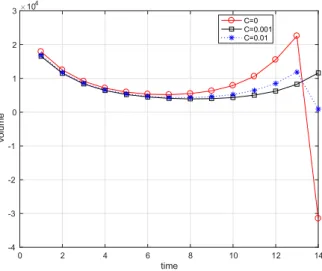
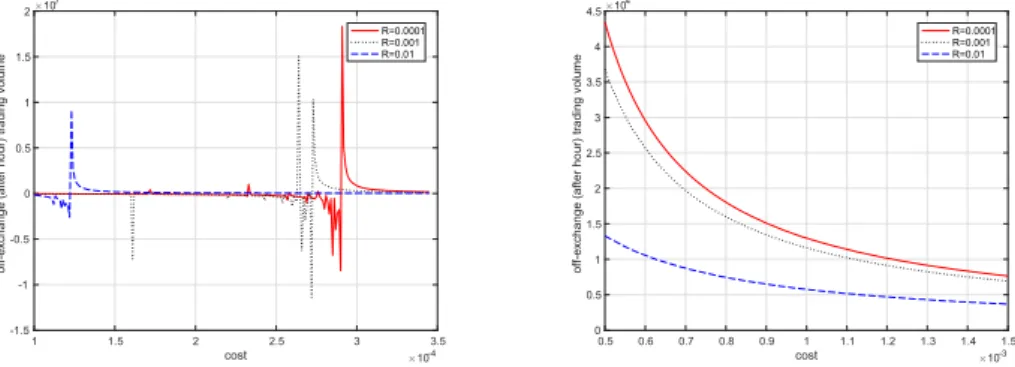
(7) 120 amount equivalent to the closing price of the day of the exchange \cros \overline{Q} units— the fee. Again the institutional investor pays a fee to the broker instead of surely obtaining \overline{Q} units at the closing price. Under such situation, we consider how much the fees that the broker sets are. That is to. say, we construct the fee systems that the institutional investor does not manipulate the market. using the argument in the previous section. Under q_{t}>0, Q_{T+1}>0 , from (2,6) and (2,7) the expected utility of the institutional investor is. V_{t}^{\pi}=E_{t}^{\pi}[-\exp\{-R(w_{T}-\hat{p}_{t}q_{t}-p_{T+1}Q_{T+1}-C_{T+1} Q_{T+1}^{2})\}|w_{t},p_{t}, Q_{t}, S_{t}, q_{t}] ,. (3.7). and from (2.8), value function is. V_{t} := \sup_{\pi}V_{t}^{\pi} .. (3.8). Q_{T+1}=\overline{Q} and determine the cost C_{T+1} as a price of the contract which achieves the. We fix. smallest under the condition of q_{t}>0, Q_{T+1}>0 . The reason to do like that, when the value of. C_{T+1} is too high, the institutional investor do not use the off‐exchange trading and the service provided by the broker do not make sense. On the other hand, the institutional investor use the off‐exchange trading as the venue of price manipulation when the value of C_{T+1} is too low.. 4. Numerical examples of institutional investor’s perspective. In this section, we present the intraday optimal execution strategy and allocation considering. both the stock exchange and the off‐exchange with comparative statics. In [11], they focused only on the allocation of both trading venues, in particular the execution strategy in the traditional exchange. We now also illustrate the execution plan in the off‐exchange explicitly and we show. that it becomes optimal for the institutional investor to manipulate the price by the level of the fee. We divide the intraday traditional stock exchange trading time into 13 periods as mentioned. in [1], and after that at time. t=T+1=14. the remaining volume is executed with market. closing price of that day. We use the following base parameters: \lambda_{t}=0.001, \alpha_{t}=0.5, \rho=0.1, \mu_{\epsilon}=0,. 4.1. \sigma_{\epsilon}^{2}=0.02, C_{T+1}=0.001,. R=0.001 ,. and \overline{Q}=100,000 unless otherwise specified.. Market impact and cost of off‐exchange. Figure 1 shows optimal execution volumes for the institutional investor if the off‐exchange trad‐. ing costs C_{T+1}=0 , 0.001, 0.01. When C_{T+1}=0 , though it seems that the institutional investor executes only at the off‐exchange, she lifts up the price on the stock exchange and sells excess her holdings in the off‐exchange. When C_{T+1}=0.001 , since it equals the market impact cost at the stock exchange then institutional investor deals the off‐exchange trading as the extension of. the stock exchange trading. Finally, it can be seen that institutional investor no longer uses the off‐exchange trading as the cost of off‐exchange trading becomes higher.. 4.2. Off‐exchange execution. Figure 2 illustrates the off‐exchange trading volume of the institutional investor. We will see that the more risk‐averse the institutional investor is, the faster she finishes her execution. In.

(8) 121 121. \supetqcir>E\omega. Figure 1: Optimal execution strategy in terms of cost. \supetqcir>E({\math}). \underli{\vap ri\subetqcir}. -L\veorline{\c supet}. \chek{fra\omeglcrn}{\udelin}varp. ‐. i\mathb{E}^frklL()xoc\vapisubet 0 02 04 06 08 1 12 14 16 18 2. cost. \cross 10^{-3}. Figure 2: Optimal off‐exchange trading volume in terms of cost.

(9) 122 any risk aversion level, the algorithm changes intensely to a certain cost level, however when. it exceeds that level, the algorithm calms down. In fact, in the low cost level the algorithm fluctuates, nevertheless it seems to be stable from Figure 2. Moreover, when C_{T+1}arrow\infty , by. equation (2.12) or [11] we get q_{T+1}arrow 0.. \frac{supetEomg}bqir\ndle{vap. \mathring{E}\veorlin{\supet-} \underli {\nfty-varpi\omega}. \mathb{E}Loegxcirvp\sutomega Figure 3: Scale up of Figure 2; 0.0001\leq C_{T+1}\leq 0.00035 and 0.0005\leq C_{T+1}\leq 0.0015 The left side of Figure 3 shows the scale up of the fluctuate part of the optimal execution at the off‐exchange in terms of the range of cost c_{\tau+1} from 0.0001 to 0.00035. We find that. as the division of the cost is finer, the optimal execution fluctuates in a certain range and it also fluctuates more intensely as the institutional investor becomes more risk‐neutral. On the other hand, the risk‐averse institutional investor will not manipulate to pursue her own profit. if the cost of the off‐exchange trading is not so low. We conjecture this fluctuation as that the range of the low off‐exchange trading cost induces the institutional investor to manipulate the. market. Indeed, the trivial changes of the market parameters cause significant fluctuations in off‐ exchange trading. In spite of using absence of manipulation price model, by adding the trading opportunity if the off‐exchange trading cost is low, algorithmic trading can make the market. unstable and under both trading venues the round trip trade would make a profit. Analytical proof and the construction of a new absence of manipulation price model are our future research. The right side of Figure 3 focuses on the range of the off‐exchange trading cost C_{T+1} around. the market impact, that is, from 0.0005 to 0.0015. As the institutional investor is more risk‐ averse, she would fasten her execution because she intends to keep away from the price change. risk. As a result, the closing price guaranteed off‐exchange execution is avoided. The point of the cost. C_{T+1}=1\cross 10^{-3} is the same as the market impact cost in the stock exchange. When. R=0.001 ,. it corresponds to time point. t=14. both \lambda_{t}=0.001 and C_{T+1}=0.001 . In this case,. the volume of the off‐exchange trading is 11,619.. 5. Concluding Remarks. The closing price guaranteed execution makes price manipulation easy by using multiple trading. venues. Under the model in [11], we showed mainly how the cost of the off‐exchange trading influenced the execution strategy of the institutional investor. The optimal execution strategies.

(10) 123 of institutional investors heavily depend on their own risk aversion and the cost of the off‐. exchange trading established by the broker. We also exemplified in particular that when the cost of the off‐exchange trading is low, the algorithmic trading by the institutional investor depending on the degree of risk aversion made the market unstable. On the other hand, if the cost was set around the market impact coefficient level, the algorithm did not cause fluctuations on the. traditional stock exchange. Actively utilize the algorithmic trading at the low off‐exchange cost reduces the overall economic welfare, which in turn can be detrimental to institutional investors. themselves. Therefore, as a precautionary measure for the price manipulation algorithm, we characterized the pricing of the guaranteed contract using closing price from the standpoint of both a broker and an institutional investor. The derivation of analytical solutions remains our future work.. References. [1] Aggarwal, R. K., and Wu, G., (Equity market impact. Journal of Business, 79, 4, 1915‐. 1953, 2006.. [2] Alfonsi, A., Schied, A., and Slynko, A., “Order Book Resilience, Price Manipulation, and the Positive Portfolio Problem. SIAM Journal on Financial Mathematics, 3, 511‐533, 2012.. [3] Almgren, A. and Chriss, N., “Optimal execution of portfolio transactions. Journal of Risk,. 3, 5‐39, 2000.. [4] Cartea, A., and Jaimungal, S. S., “A Closed‐Form Execution Strategy to Target Volume Weighted Average Price. SIAM Journal on Financial Mathematics, 7, 760‐785, 2016.. [5] Gatheral, J., “No‐dynamic‐arbitrage and market impact. Quantitative Finance, 10, 7,. 749‐759, 2010.. [6] Guéant, O., and Royer, G., “VWAP Execution and Guaranteed VWAP. SIAM Journal. on Financial Mathematics, 5, 1, 445‐471, 2014.. [7] Hillion, P., and Suominen, M., “The manipulation of closing prices. Journal of Financial. Markets, 7, 351‐375, 2004.. [8] Huberman, G., and Stanzl, M., “Price Manipulation and Quasi‐arbitrage. Econometrica,. 72, 1247‐1275, 2004.. [9] Kratz, P., and Schöneborn, T., “Optimal liquidation in dark pools. Quantitative Finance,. 14, 9, 1519‐1539, 2014.. [10] Kuno, S., and Ohnishi, M., “Optimal Execution in Illiquid Market with the Absence of Price Manipulation. Journal of Mathematical Finance, 5, 1, 1‐14, 2015.. [11] Kuno, S., Ohnishi, M., and Shimizu, P., “Optimal Off‐Exchange Execution with Closing Price. Journal of Mathematical Finance, 7, 1, 54‐64, 2017..

(11) 124 [12] Mittal, H., “Are You Playing in a Toxic Dark Pool? A Guide to Preventing Information Leakage. Journal of Trading, 3, 20‐33, 2008.. Faculty of Commerce, Doshisha University Kamigyo‐ku, Kyoto, 602‐8580 Japan E‐mail address: [email protected].

(12)