Ultradiscrete Soliton Systems and Combinatorial Representation Theory (Algebraic Combinatorics related to Young diagram and statistical physics)

UItradiscrete Soliton Systems

and

Combinatorial

Representation

Theory

${\rm Re}\dot{\ovalbox{\tt\small REJECT}}ho$

Sakamoto

Department$\mathfrak{o}fPhys\dot{\ovalbox{\tt\small REJECT}}cs$

, Tokyo

University

of$Sc\dot{\ovalbox{\tt\small REJECT}}$

ence, Kagurazaka $Sh\dot{\ovalbox{\tt\small REJECT}}$

njukuku Tokyo Japan

1

Introduction

This lecture note is intended to be a brief introduction to a recent development on the interplay between the ultradiscrete (or tropical) soliton systems and the combinatorial representation theory. We will concentrate onthe simplest

cases

which admit elementary explanations without losing essential ideas of the theory. In particular wegive definitions for the main constructions corresponding to the vector representation of type $A_{1}^{(1)}.$

This note is organized as follows. In Section 2 we give a definition ofthe simplest ex-ample ofthe box-ballsystems. InSection

3 we

explain

a

relationship between the box-ball systems and the crystal bases of the quantum affine algebras. In

Section 4 we

give the definition of the rigged configuration bijection for the vector representation oftype $A_{1}^{(1)}.$

In Section 5 we see that the riggedconfigurations give the complete set of the action and angle variables for the box-ballsystems. This is thefundamental observation in the recent development on a relationship between the box-ballsystems and thecombinatorial

repre-sentationtheory. In Section 6

we

explain basic properties ofthe box-basket-ball systems

which

are

recently found generalizations of the box-ball systems. The characteristic prop-erty of the system is that it is a mixture offermions and bosons with mutual interactions. Finally, in Section 7,

we

give comments

on

generalizations and further developments of the materials discussed in this note.

This is the lecture note prepared for the conference “Algebraic Combinatorics related to Young diagram and statistical physics” held at International Institute for Advanced Studies (Kyoto) during August 6-10,

2012.

The author is grateful to Professor Masao Ishikawa, Professor Soichi Okada and Professor Hiroyuki Tagawa for the kind invitation to the conference and the

warm

hospitality.

2

The

box-ball

systems

In this section, let

us

define the simplest

case

of the box-ball systems introduced by Takahashi and Satsuma [TS]. The box-ball systems are prototypical examples of the ultradiscrete soliton systems. Originally the ultradiscrete soliton system is

a

class of discrete dynamical systems obtained by the ultradiscrete (or tropical) limitof the ordinary soliton systems [TTMS]. In this article

we

are interested in ultradiscrete soliton systems which admit combinatorial interpretations.

Following the box and ball interpretation of the system [T3],

we prepare

boxes which

can

accommodate at most

one

ball within each box. We put many such boxes

on a

line and put finitely many balls of the

same

kind to the boxes. We regard this configuration asthe initial state of the system. Then we perform the time evolution of the state by the following algorithm.

The time evolution ofthe box-ball system: Consider each ball from left to right and

move

the ball to the next

available

empty box.

Each

ball is moved exactly

once.

Hereifnecessarywe put enoughmanyempty boxesonthe right of the givenstateinorder to keep the balls within the state. We give an example of such time evolution starting from the top

row

and proceeding downwards.

Inthe box-ball system,

we

regardconsecutiveballs

as

solitary

waves.

For example, the ini-tial state in the above examplecontainstwosolitary waves of length3 and 1, respectively. Then our interpretation of the above example is

as

follows. If there is

no

interaction between waves, they

move

at velocity equal to each length. In the

course

of the time evolution, solitary

waves

make collision with each other, though theyretain their original shapes after the collision except for the changes in the positions compared with the pos-sible positionswe would have if there isno interaction between

waves.

Such properties of the waves of the box-ball systems

are

characteristic of the soliton systems (see, e.g., [T4]) and

we

will call such

waves

solitons.

Here

we

give

a

short list of remarks

on

the early

papers.

During $1980’ s$, there

were

several attempts of findingcellular automata with solitonic properties. A typical example of such researchesis thefilter automata introducedbyPark, Steiglitz andThurston [PST]. In 1990, Takahashi and Satsuma [TS] introducedthe simplest

case

ofthe box-ball systems and Takahashi [T3] described the algorithm in terms ofthe boxes and balls. The above definition corresponds to the original Takahashi-Satsuma box ballsystem. A relationship

between theTakahashi-Satsuma box-ballsystem and the ordinary soliton systems includ-ing the $KdV$ equation is discovered by Tokihiro, Takahashi, Matsukidaira and Satsuma

[TTMS] via the limiting procedure called the ultradiscrete limit. A connection with the Toda equation is discussed in [NTT]. Such connections between the box-ball system and the usual soliton systems show the classical integrability of the box-ball system.

Takahashi’sbox and ball algorithm provides several generalizations of the original box-ball system. For $exam\iota\rangle$}$e$, in [T3]

an

internal degree of freedom for the balls (balis with

different colors) is introduced. A connection with the Toda equation in the generalized context is discussed in [TNS]. The other degrees of freedom called a carrier [TM] or a capacity of boxes [TTM]

are

also introduced. Such combinatorial interpretations of the time evolutions give nice intuition about the models in many

cases.

3

A

connection

with

the

crystal

bases

A veryimportant fact [HHIKTT, FOY] about the box-ball systems is that their dynamics is infactgoverned by the Kashiwara’s crystal bases [K2] forthe quantumaffine algebras. This formalism includes all extensions of the box-ball system which

are

mentioned in the last section. Although the formulation does not depend on the types ofthe algebra, we will concentrate on the simplest

case

$A_{1}^{(1)}$

here.

In order to describe the formulation, we need to consider more general boxes which

have capacities more than one. Let $(a, b)$ represents the box of capacity $a+b$ containing

$b$ balls. Then the state _{$(a, b)$}

can

accommodate extra_$a$ balls. Let

us

denote the set of all

such states

as

$B^{1,s} :=\{(a, b)|a, b\in \mathbb{Z}_{\geq 0}, a+b=s\}$ (1)

which we call

crystals.1

In particular we call $B^{1,1}$ the crystals for the vector

repre-sentation. In this coordinate, the states of the box-ball system in the previous section

are

sequences of balls $(0,1)$ _and empty _places $(1, 0)$. Then

we

represent the states

as

$(1, 0)\otimes(0,1)\otimes\cdots$ where $\otimes is$ the tensor product ofcrystals (thereaders may regardthis

asjust alternativenotation). We call such elements of tensor products paths.

The main ingredient of the formalism is the map called the combinatorial$R$-matrices $R$ : $B^{1,s}\otimes B^{1,s’}$ $arrow$ $B^{1,s’}\otimes B^{1,s}$

(2)

$(a, b)\otimes(c, d) \mapsto (c’, d’)\otimes(a’, b$

In the present

case

$A_{1}^{(1)}$

, the explicit form of the map is

$a’=a+ \min(b, c)-\min(a, d)$

$b’=b- \min(b, c)+\min(a, d)$ $c’=c- \min(b, c)+\min(a, d)$

$d’=d+ \min(b, c)-\min(a, d)$. (3)

An important point of the map $R$ is that it has a deep mathematical origin as the inter-twining map that interchanges left and right of the tensor products of crystals. For the laterpurposes we introduce avertex diagram for the map $R:a\otimes b\mapsto b’\otimes a’$

as

follows:

1In general, we can identify the Kirillov-Reshetikhin crystals $B^{r,s}$ for type $A_{n-1}^{(1)}$ with the set of $r\cross s$ semistandard tableauxwith letters 1, 2,...,$n$. In this identification our $(a, b)$ is the height one

semistandard tableau with$a$ $1$’sand_{$b2’ s.$} $B^{r,s}$ corresponds to the Kirillov-Reshetikhin module naturally

$a+_{b’}^{b}a’.$

By a repeated

use

of the map $R$ we define the time evolution of the box-ball systems

$T_{l}(l\in \mathbb{Z}_{\geq 1})$

as

follows. Let $u_{l}$ $:=(l, 0)$ be the empty box of capacity

$l$ and let $b=$ $b_{1}\otimes b_{2}\otimes\cdots\otimes b_{L}$ be

a

given state of the box-ball system. We call $u_{l}$ the carrier. If

necessary

we

put enough many empty boxes $(1, 0)$

on

the right. Then we define $b_{1}’$, .

.

.,

$b_{L}’$ by the following diagram.

(4) Here the precise meaning of the diagramis

as

follows. We compute$R$ : $u_{l}\otimes b_{1}\mapsto b_{1}’\otimes u_{l}^{(1)}.$

Then by using$u_{l}^{(1)}$ we compute $R:u_{l}^{(1)}\otimes b_{2}\mapsto b_{2}’\otimes u_{l}^{(2)}$. We dothis procedure recursively

until the end ofthe state. Then

we

define

$T_{l}(b):=b_{1}’\otimes b_{2}’\otimes\cdots\otimes b_{L}’$. (5) We

can

see that the time evolution rule given in Section 2 coincides with $T_{\infty}$ here.

As a benefit of the definition by the crystal bases, we can show the quantum inte-grability of the box-ball system

as

the consequence of the Yang-Baxter relation for the combinatorial $R$-matrices [FOY]. More precisely, we have

$T_{l}T_{k}(b)=T_{k}T_{l}(b)$ (6)

for arbitrary $l,$ $k\in \mathbb{Z}_{\geq 1}$ and states $b$. Moreover,

we

can construct conserved quantities of

the box-ball system

as

follows. Let

us

define (see(4))

$E_{l}(b) := \sum_{i=1}^{L}H(u_{l}^{(i-1)}\otimes b_{i}) , E_{0}(b) :=0$ (7)

where $u_{l}^{(0)}$

$:=u_{l}$ and the energy function $H:B^{1,s}\otimes B^{1,s’}arrow \mathbb{Z}$ is defined by

$H((a, b) \otimes(c, d)) :=\min(a, d)$. (8)

Again

an

important point of the

energy

function is that it has

a

deep mathematical origin and is the consequence of the infinite dimensional symmetry of the quantum affine algebras. Let

us

consider the affinization ofthe crystal $B$

For

elements

of tensor products

of

$Aff(B)$_,

_we

_{introduce the affine}

_{combinatorial}

R-matrices by

$R_{aff}$ : $b_{1}[d_{1}]\otimes b_{2}[d_{2}]\mapsto b_{2}’[d_{2}-H(b_{1}\otimes b_{2})]\otimes b_{1}’[d_{1}+H(b_{1}\otimes b_{2}$ (10) wherewehave$R:b_{1}\otimes b_{2}\mapsto b_{2}’\otimes b_{1}’$ under the combinatorial$R$matrix. Then by the Yang-Baxter relation for the affine combinatorial $R$-matrices we see that $E_{l}$ are the conserved

quantities ofthe box-bail systems [FOY]:

$E_{l}(T_{k}(b))=E_{l}(b)$. (11)

4

The rigged configurations

Another important aspect ofthe box-ball systems is

a

connection with the rigged config-urations. In this section we give thedefinition of a specialcase of the rigged configuration bijection corresponding to the vector representation of type $A_{1}^{(1)}$

. Although this case is simpler than the generalcase, it is still nontrivial and we can see basic ideas ofthe theory. Originally the rigged configurations

are

discovered through insightful analysis of the Bethe ansatz for quantum integrable systems [KKR, KR]. The main ingredient of the theory is a bijection between the set of rigged configurations and elements of the tensor

products of crystals. Such a bijection is generalized for highest weight elements of tensor

products of the arbitrary Kirillov-Reshetikhincrystals of type $A_{n}^{(1)}$

and its mathematical theory is established by

an

important paper of Kirillov, Schilling and Shimozono [KSS].

In our case, a rigged configuration is composed of a Young diagram (called the

con-figuration) and integers (called the riggings) associated with each

row

of the Young diagram. Let $\nu_{i}(i=1, \ldots, g)$ be the lengths of the

rows

ofthe configuration and let $J_{i}$

be the rigging associated with the

row

$v_{i}$. Then we represent the rigged configuration as

$(\nu, J)=\{(\nu_{i}, J_{i})\}_{i=1}^{g}$. We call each $(\nu_{i}, J_{i})$ string. Although there is a characterization

ofthe possible rigged configurations, we regard the set of the rigged configurations

as

the set of objects obtained by the map (in fact, bijection)

$\Phi:b\mapsto(\nu, J)$ (12)

from arbitrary paths $b$. We call the bijection $\Phi$ the rigged configuration bijection.

Let us define the algorithm of the bijection $\Phi$. For the given Young

diagram $\nu$ let $Q_{\ell}(v)$ be the numberof boxes contained-in the left $\ell$

columns of $\nu$. Suppose that we are

given the path$b=b_{1}\otimes b_{2}\otimes\cdots\otimes b_{L}\in(B^{1,1})^{\otimes L}$ wherethe positions of the balls _{$b_{k}=(0,1)$}

are

given by $k=k_{1},$$k_{2}$,. . . from left to right. Let _{$P_{\ell}(k, \nu)$} be the vacancy number

defined by

$P_{\ell}(k, \nu):=k-2Q_{\ell}(\nu)$

.

(13)

For example, we have $P_{2}(16, \ovalbox{\tt\small REJECT})=16-2\cdot 5=6$. Suppose that a length $L$ path $b$

corresponds to the rigged configuration $(\nu, J)$. Then we call the string $(\nu_{i}, J_{i})$ singular if

the rigging $J_{i}$ coincides with the corresponding vacancy

number, that is, $P_{\nu_{i}}(L, \nu)=J_{i}.$ The bijection $\Phi$

is defined by a recursive procedure corresponding to the positions of balls $k_{1},$$k_{2}$, .. .. We start from the empty rigged configuration.

1. Suppose

that we have

done the

procedure up

to$k_{j-1}$ and

obtained

the

intermediate

rigged configuration $(\eta, I)$.

2. For the next position $k_{j}$, we do the following. Suppose that the rigged configuration

$(\eta, I)$ corresponds to a length $k_{j}-1$ path. Compute the vacancy numbers $P_{\eta_{i}}(k_{j}-$ $1,$$\eta)$ for all rows of$\eta$ and determine all the singular strings.

3.

If there is

no

singular string, add

a

length

one row

to the bottom of $\eta$

.

Otherwise

choose

one

of the longest singular string and add

a

box to the corresponding

row.

Denote by$\eta’$ the new configuration thus

obtained.2

4. Define the new rigging $I’$ as follows. For the strings that

are

not changed under $\etaarrow\eta’$, we choose the same riggings as before. Let $\eta_{i}’$ be the changed

row

under

$\etaarrow\eta’$

.

Then

define

the

new

rigging by $I_{i}’=P_{\eta_{i}’}(k_{j}, \eta’)$

so

that the string $(\eta_{i}’, I_{i}’)$ is

singular in $(\eta’, I The$ output $(\eta’, I’)$ isthe

new

rigged configuration corresponding to the length $k_{j}$ path.

5. Repeat the

same

procedure for all $k_{j}$. Let $(\nu, J)$ be the final output. Then define

$\Phi(b)=(\nu, J)$.

A Mathematica package for the above procedure is available at [S3]. If

we

reverse

all the procedure

we

obtain the algorithm for $\Phi^{-1}$. As

examples, let

us

look at the example of the time evolution of the box-ball system at Section 2. In the first line, the positions of balls $k_{j}$

are

1, 2, 3,8. Then the computation of $\Phi$ proceeds

as

follows:

$\emptysetarrow 1$

(14) Here

we

put riggings

on

the right of the corresponding

row

and put $k_{j}$ above the

corre-sponding arrows. Similarly, for the third line of the same example, we have

$\emptysetarrow 7$

(15)

5

The

inverse scattering formalism

The main observation on the relationship between the rigged configurations and the

box-ball systems is that the rigged configuration bijection gives the inverse-scattering

formal-ism for the box-ball systems. In order to get the ideas of the result, let

us

compare the two examples in (14) and (15). Then we

see

that the shapes of the configurations are

same

and the differences of the riggings

are

two times the lengths of the corresponding

rows.

Here

we

have the factor 2 in the change ofriggings since we apply $T_{\infty}$ twice.

In general, let $b$bethegivenstate and let $\Phi(b)=\{(\nu_{i}, J_{i})\}_{i=1}^{g}$. Thenwehave [KOSTY]

$\Phi(T_{l}(b))=\{(\nu_{i}, J_{i}+\min(l, \nu_{i}))\}_{i=1}^{g}$. (16)

This property is valid for general box-ball systems including all

cases

that appeared in [HHIKTT, FOY]. The proof of this fact heavily relies on a deep theorem of Kirillov-Schilling-Shimozono [KSS].3 Indeed, if

we

compare (14) and (15) we

can see

that this property is already nontrivial. To summarize, configurations are the conserved quantities (action variables) and the riggings

are

the linearlization parameter (angle variables) of the box-ballsystems. Since $\Phi$ is bijective, the rigged configurations give the complete set

ofthe action and angle variables of the box-ball

systems.4

Once we know that the rigged configurations are the underlying mathematical struc-ture of the box-ball systems,

we can

prove several fundamental properties of the box-ball systems. For example, the box-ball systems considered in [HHIKTT, FOY]

are

shown to be solitonic byintroducing a method to explicitly extract solitons from paths

as

elements of the affinization of the crystals [S1]. The main point of the proof of the result is to introduce a structure of the affine combinatorial $R$-matrices on the rigged configurations viacareful combinatorial arguments. We remark that the proof of the solitonic properties of the box-ball systems corresponding to the vector representation of type $A_{n}^{(1)}$

is proved in [TNS] bytaking certainultradiscretelimit ofanordinary soliton system and

an

elegant alternative proofoftheir result is given in [FOY] by using the crystal bases.

Another important problem that is solved by the rigged $config_{UT}$ation bijection is

the initial value problem of the box-ball systems [KSYI]. The result includes all the extensions considered in [HHIKTT, FOY]. We note that an equivalent result for the

case

of the vector representation of$A_{1}^{(1)}$

is rederived in [MIT2]. Let

us

explain the result for the

case

of the vector representation of $A_{1}^{(1)}$

. The main point is to give

an

explicit piecewise linearformulafor the map$\Phi^{-1}$ : _{$(\nu, J)\mapsto b$}.

Forthegiven riggedconfiguration

$(\nu, J)=\{(\nu_{i}, J_{i})\}_{i=1}^{g}$, let us define the following ultradiscrete tau functions:

$\tau_{r}(k)$ _{$:=- \min_{n\in\{0,1\}^{g}}\{\sum_{i=1}^{g}(J_{i}+r\nu_{i}-k)n_{i}+\sum_{i,j=1}^{g}\min(\nu_{i}, \nu_{j})n_{i}n_{j}\},$} $(r=0,1)$ (17)

where

we

denote $n=(n_{1}, \ldots, n_{g})^{5}$ Let us represent the k-th element of the path $b$

as

$b_{k}=(1-x(k), x(k))$. Then we have the following analytic expression for the image $b$: $x(k)=\tau_{0}(k)-\tau_{0}(k-1)-\tau_{1}(k)+\tau_{1}(k-1)$. (18)

3Iftwo tensor products $b$ and $b’$ are isomorphic under the combinatorial $R$-matrices $R$ : $b\mapsto b’$, we

have $\Phi(b)=\Phi(b’)$ [KSS, Lemma8.5]. Theproof depends on a _large part of the paper.

4In fact ifwe restrict to consider the box-ball systems corresponding to the vector representation

of type $A_{1}^{(1)}$,

we do not need to use heavy apparatus like rigged configurations. For example, [TTS] introduced a combinatorialmethod to obtain the conserved quantities. In [MITI], amethod to obtain the action and angle variables is derived, which is shown to be the specialcaseof the rigged configurations [KS1]. In [KOTY] it is conjectured that the rigged configurations give the action and angle variables of thebox-ballsystem corresponding to the vectorrepresentationof type$A_{1}^{(1)}$. This problem is considered in [T1] with differently definedbijection. We remark that in [F] the Robinson Schensted-Knuthalgorithm

is used to give some of the conserved quantities of the box-ball system corresponding to the vector representationsof type $A_{n}^{(1)}$

(socalled $P$-symbolsare _{conserved under the time evolutions).}

5Ifwe consider paths with periodicities, these functions $\tau_{r}$ exactlycoincide with the tropical

Since

the time evolution of the box-ball system is linearlized

on

the set of the

rigged

configurations, this result gives

an

explicit solution for the initial value problem of the box-ball systems.

Sketch

_of

the proof

_of

(18). The mainstepof theproof is to show the following interpreta-tion ofthe taufunctions. For thegiven path$b=b_{1}\otimes b_{2}\otimes\cdots$, define$T_{\infty}(b)=b_{1}^{(1)}\otimes b_{2}^{(1)}\otimes\cdots,$ $T_{\infty}^{2}(b)=b_{1}^{(2)}\otimes b_{2}^{(2)}\otimes\cdots$ , and so on. Then we have to show the following interpretation:

$\tau_{r}(k)=(1-r)\cross($number of balls in $b_{1}\otimes b_{2}\otimes\cdots\otimes b_{k})$

$+ \sum_{i\geq 1}$(number of balls in

$b_{1}^{(i)}\otimes b_{2}^{(i)}\otimes\cdots\otimes b_{k}^{(i)}$). (19)

For example, in the example of Section 2,

we

have $\tau_{0}(8)=9$ and $\tau_{1}(8)=5$. Since balls

always

move

rightwards, the summation in the second term is always finite. From (19)

we

can

easily deduce (18).

Proof of(19) proceeds as follows. From the expression (17) we canconstruct determi-nantsfrom which

we

obtain thetau functions $\tau_{r}$

as

theultradiscrete limit. Then by using

a calculus of determinants we

can

show that the tau functions satisfy the ultradiscrete Hirota bilinear form. The Hirota bilinear form implies that the functions $\tau_{r}$ corresponds

to the

same

dynamics of the box-ball systems. Unfortunately this is not thewhole story. The main difficulty is the fact that the analytic expression in (17) is very different from the

$Wedothisinthef$

Sincecombinatorial

ollowing

w

$ay.Thep$roof i$si$nduction

o

$ntheranknofA_{n}^{(1)}.$

definition o$fthemap\Phi^{-1}andthusitisq$uite difficult t$\circ$ compare.

we know that the tau functions satisfy the

same

dynamics of the box-ball systems, it is enough to consider

a

state $T_{\infty}^{N}(b)$ where $N\gg 1$. We call such

a

state the asymptotic

state. Since we have the inverse scattering formalism which is the consequence of the most part of the paper [KSS],

we can

easily obtain the corresponding asymptotic rigged configuration. Then weinvoke the result of [S1] to reducethe problem to the

case

of$A_{n-1}^{(1)}$ (the

case

$A_{1}^{(1)}$

can

be shown by [S1]). This part is logically

a

bit complicated and

we

will omit the details. Here

we

remark that

we

use

the fact that the tau functions for the general $A_{n}^{(1)}$

have

a

similar recursive structure with respect to the rank and that we

use

the Yang-Baxter relations for the affine combinatorial $R$-matrices to represent the right hand side of (19) by the energy function and the combinatorial $R$-matrices. Thus the proof heavily utilizes the infinite dimensional symmetry behind the box-ball system. $\square$

Finally

we

remark that the conserved quantities $E_{l}$ of [FOY] indeed coincide with the

rigged configurations [S2]:

$E_{l}(b)=Q_{l}(\nu)$ (20)

where $\Phi(b)=(\nu, J)^{6}$ There is ageneralization of this formula for the most general rigged

6In [T2], Takagi introduced ascheme to factorize thedynamics ofthebox-ball systemsoftype $A_{n}^{(1)}$ into $A_{1}^{(1)}$ case by using the time evolution corresponding to the carrier of type $B^{2,1}$. _{This scheme is} rephrased intotherigged configuration language [KOSTY, Section2.7] to factorize the map$\Phi$forgeneral

$A_{n}^{(1)}$

case into the map $\Phi$ for $A_{1}^{(1)}$ casebyusing the $B^{2,1}$ _{type time evolution. The proof of (20) in [S2]}

configuration bijectionoftype $A_{n}^{(1)}$

(seeSection7). By (20) wesee that the configurations have a simple representation theoretical origin in terms of the combinatorial $R$-matrices and the energy function. In fact, in [S2] it is shown that the quantities $E_{l}$ (and suitable

refinements) give enough information to reconstruct riggings. In this sense, the combina-torial algorithm of$\Phi$ itselfhas arepresentation theoretical

origin via the time evolutions of the box-ball systems. However the mathematical origin of the riggings is still unclear. In fact, the riggings depend

on

the

information

about the final positions where the

cor-responding string is finally changed during the procedure $\Phi$. This information

is rather combinatorial and we cannot get rid of its difficulty

even

if

we

use the representation

theoretical interpretation ofthe algorithm of $\Phi$ discussed

above.

6

Interlude:

the

box-basket-ball

systems

In this section, we explain the basic properties of the box-basket-ball systems (BBBS

for short) introduced by [LPS]. The starting point of the construction is to replace the combinatorial $R$-matrices in the definition of the box-ball system by the whurl _relations of [LP]. Rather non-trivially, the resulting dynamical system becomes

a

soliton system.

The

characteristic

property of the

BBBS

is that the system contains the

fermions

(balls)

and bosons (baskets) with mutual interaction between them. We remark here that the BBBS is different from thesuper-symmetric box-ballsystem of [HI] constructed from the crystals for the quantum superalgebra [BKK] since their system is the extension of the box-ball system by adding another kind of the fermionic particles.

In order to obtain intuition about the model, it is convenient to start from a com-binatorial description of the time evolution of the BBBS. Let $b=b_{1}\otimes b_{2}\otimes\cdots$ be the state of the BBBS. In this situation, each state is parametrized

as a

three dimensional vector $(a, b, c)\in \mathbb{Z}^{3}$. Our interpretation of each parameter is as follows; $b$ is the number

of baskets, $c$ is the number ofballs and $a$ is the number ofempty places that can fit

extra balls. The meaning of such an interpretation will become clearwhen

we

explain the combinatorial description of the time evolution.

In the rest of this section,

we

consider the following situation. Weput many capacity

one

boxes

on a

line. If necessary,

we

put enough many empty boxes on the right of the state. As the rule, each box

or

basket

can

accommodate at most

one

ball whereas we can put more than one baskets on abox. Thus the balls are fermionic particles and the baskets are bosonic particles. There is anontrivial interaction between the two kinds of

particles by placing a ball within a basket. Ifnecessary we

assume

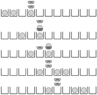
that a ball is always

placed in a box before placed in a basket. We introduce several definitions that will be used later. Let $V=(1,0,0)$, $F=(0,0,1)$, $B_{i}=(i+1, i, 0)$ and $U_{i}=(i, i, 1)$ where $i\geq 1.$

Here we give several diagrams that represent these symbols:

$V=\sqcup, F=\sqcup, B_{2}=\sqcuprightarrow\Leftrightarrow, U_{2}= \sqcup\ovalbox{\tt\small REJECT}\ovalbox{\tt\small REJECT}\Leftrightarrow.$

Now

we

explain the time evolution rule. We start from an initial state that contains finitely many baskets and balls.

$\sqcup Q\sqcup\sqcup\sqcup\sqcup\sqcup\sqcup\sqcup\sqcup\sqcup\sqcup\Leftrightarrow\Leftrightarrow$ $u\sqcup\sqcup\sqcup\sqcup\sqcup\sqcup\sqcup\sqcup\sqcup\sqcup\bigotimes_{\bullet}^{\Leftrightarrow}$ $\mathfrak{B}$

@

$\sqcup\sqcup\sqcup\sqcup\sqcup\sqcup\sqcup\sqcup\sqcup\sqcup\sqcup$ $rightarrow$ $\sqcup\sqcup\sqcup\sqcup\sqcup\sqcup\sqcup Q\sqcup\bullet\sqcup\sqcup\sqcup\Leftrightarrow$ $\approx$ $\sqcup\sqcup\sqcup\sqcup\sqcup\sqcup\sqcup\sqcup\sqcup\sqcup\sqcup\Leftrightarrow$

Figure 1: Example ofthe time evolution of the BBBS.

The time evolution of the

BBBS:

First,

move

every empty basket to the right one step. Full baskets

are

not moved. Second, consider each ball from leftto right and

move

the ballto thenext availableemptybox

or

basket. Each ball is moved exactly

once.

Note that if there is

no

basket, the above rule coincides with the

one

for the box-ball system. We give

a

simple but nontrivial example in Figure 1.

The BBBS

can

be constructed from the whurl relation

$R:(a, b, c)\otimes(d, e, f)\mapsto(d’, e’, f’)\otimes(a’, b’, c’)$ (21)

where the explicit relations

are

$a’=a- \min(a+b, a+c, b+f)+\min(e+c, d+c, d+b)$ $b’=b- \min(a+b, a+c, b+f)+\min(a+e, d+f, e+f)$ $c’=c- \min(e+c, d+c, d+b)+\min(a+e, d+f, e+f)$

$d’=d+ \min(a+b, a+c, b+f)-\min(e+c, d+c, d+b)$

$e’=e+ \min(a+b, a+c, b+f)-\min(a+e, d+f, e+f)$

$f’=f+ \min(e+c, d+c, d+b)-\min(a+e, d+f, e+f)$. (22) We apply the whurl relation with $u_{l}$ $:=(l, 0,0)$ to the diagram (4) to define the operators $T_{l}(l\in \mathbb{Z}_{l\geq 1})$. Then

we can

show that the above mentioned combinatorial definition of

the time evolution coincides with $T_{\infty}$. Since the whurl relations satisfy the Yang-Baxter

relation,

we can

show that $T_{l}T_{k}(b)=T_{k}T_{l}(b)$ for arbitrary $l,$$k\in \mathbb{Z}_{\geq 1}$ and states $b$. Thus

the underlying symmetry of the whurl relations, we have not been able to construct a conserved quantity analogous to $E_{l}.$

Even if

we

know that the

BBBS

is

a

quantum integrable system, it is far from clear whether the system is a soliton system. Below we explain that the system is indeed solitonic. For this purpose we classify solitary

waves

which do not change their shapes during the free propagations under$T_{\infty}$. As the result, we

see

that there

are

the following

two

cases.

1. A consecutive sequence of $k$ balls $F_{k}$ $:=FF\cdots F$

.

Under the free propagation by

$T_{\infty},$ $F_{k}$

moves

at velocity $k.$

2. Any sequence of $F,$$B,$$U$ which does not contain the consecutive subsequence _$FF$ or $FU$, which we _calla _{slow soliton. Under the free propagation by} $T_{\infty}$, the slow

solitons

move

at velocity 1.

Note that $F_{k}$

are

the usual

solitons

of the box-ball system

whereas

the slow solitons

are

the

new

feature of the

BBBS.

Let us clarify what

are

the slow solitons. The

answer comes

from the analysis ofthe phase shift. Here the meaning of the phase shift is

as

follows. Let $A$ and $B$

are

solitons

on

a line and suppose that they make collision during the time evolution and retain their original form after the collision. Then we compare the position of the soliton after the collision with the position ofthecorrespondingsolitonsupposing that there is

no

collision. This difference (rightwardsshift ispositive) givesthephaseshift. We summarize the basic physical properties of the fermionic solitons $F_{k}$ and the bosonic solitons $B_{a_{1}}B_{a_{2}}\cdots B_{a_{m}}$ in

the following table.

Here the phase shift is defined by the scattering with $F_{l}(l>k)$. For example, in the

example in Section 2, we see that the length one soliton $F_{1}$ get shifted by $-2$ after the

collision with $F_{3}^{7}$

Let

us

look at two solitons $F_{1}$ and $B_{i}$ of velocity one. If we consider the scattering

with $F_{k}(k>1)$, they get shifted _by $-2$ and $-1$_, respectively. To summarize, $F_{1}$ and $B_{i}$

have the

same

velocity whereas theyhave different values ofthe phaseshift. Thus during the time evolutions we may have superposition of suchstates and this is the originofthe slow solitons. Therefore, in order to analyze the slow solitons, we make scatterings with 7Letusmentionthe generalizationstothebox-ballsystemsofthevectorrepresentationsfortypes$A_{n}^{(1)}.$

Then it is known that thephaseshift coincides with the energy function (witha different normalization)

betweentwosolitons [FOY]. Hereweidentify freely propagatingsolitonswith the semistandardtableaux and regard them as the elements of crystals $B^{1,s}$ _{of types} $A_{n-1}^{(1)}$. Note that since we are neglecting all l’s (empty places), we have $A_{n-1}^{(1)}$

here. In [S1], it is generalized to include all cases considered in [HHIKTT, FOY] and the scatterings ofsoitons are identified with the affine combinatorial $R$-matrices (10) whereeach $soh^{-}ton$_{corresponds to the truncated} $r\overline{l}$

many $F_{k}$’s and decompose them into elementary solitons $F_{1}$ and $B_{i}$

.

For example, the

example in Figure 1 shows the decomposition of the slow soliton $U_{2}$ into two elementary

solitons $F_{1}$ and $B_{2}.$

Based on

these observations,

we define the solitons of

the states of

the BBBS

as

the

elementary solitons $F_{l}$ and $B_{i}$ which we

can

obtain by scattering with many

additional

$F_{k}’ s$. Let

us

define the amplitudes of$F_{l}$ and$B_{i}$ by $l$ and$i$, respectively. Then

we can

show

that thenumberand amplitudes ofthe solitons

are

preserved during the time evolutionof the BBBS. Moreoverwe

can

show that scatterings of multiple solitons

can

bedecomposed into two body scatterings. Hence we

see

that the BBBS is solitonic.

7

Generalizations and further

developments

In the most of the present note, we only think about the simplest possible case, namely the vector representation of type $A_{1}^{(1)}$

.

We do

so

in order to provide the basic ideas

without getting into the

technical

complexities. In fact,

one

of the nice features of

our

approach is its universality. For example, the

definition

of the

box-ball

system in (4) has straightforward generalizations forthetensor productsoftheKirillov-Reshetikhin crystals

$B^{r,s}$ for the quantum affine algebras of types other than $A_{n}^{(1)}$

.

Here $B^{r,s}$ is the

Kirillov-Reshetikhin crystals corresponding to the weight $s\Lambda_{r}$, where $\Lambda_{r}$ is the r-th fundamental

weight. In this case, instead of using $u_{l}$ in (4),

we

use the classically highest weight

element of$B^{r,s}$

.

Then

we

denote by$T^{r,s}$ the resultingtime evolutions. Again thebox and

ball interpretation of the time evolution provides

a

nice way to get intuition about the generalized models. For example, for the box-ball systems corresponding to the vector representations of general non-exceptional affine algebras, there is an interpretation of

$T^{1,\infty}$ in terms of particles and anti-particles with pair creations/annihilations [HKT]. In

thisfinalsection, wewill givecomments on the methods of the generalizations and further properties.

Known extensions. The rigged configuration is known to have many extensions. In-deed it is expected that such a bijection exists for the arbitrary Kirillov-Reshetikhin crystals corresponding to general affine quantum algebras. As mentioned in Section 4, the bijection for type$A_{n}^{(1)}$

is already constructedinfull generalities. Apartfrom this case, we have the following generalizations.

$\bullet$ $\otimes B^{1,1}$ for arbitrary non-exceptional affine algebras [OSS2].

$\bullet$ $\otimes_{i}B^{r_{i},1}$ for type $D_{n}^{(1)}$ [S4].

$\bullet$ $\otimes_{i}B^{1,s_{i}}$ for type $D_{n}^{(1)}$ [SS].

$\bullet$ $B^{r,s}$ of type

$D_{n}^{(1)}$

[OSSI].

We

remark that the combinatorial algorithms involved in these extensions share many

common

features and the philosophy which underlies these extensions is the same. We also remark that all these results

are

related with the highest weight elements of tensor products of crystals. However, if

we

think about the box-ball systems

we

encounter the rigged configurations for not necessarily highest weight elements. This extension is quite

natural. Indeed thealgorithmpresented in

Section 4

does applyto both

cases

withoutany change. Thereforeit is quitenatural to consider the Kashiwara operators (analogueofthe Chevalley generators in the crystals setting) on the set ofthe rigged configurations. This is achieved in [S5] for allsimply laced cases. Remarkably, the definition of the Kashiwara operators for the all

cases

considered in [S5] is uniform.

The method of generalizations. As examples of the generalizations, let

us

consider the

cases

$A_{n}^{(1)}$

or

$D_{n}^{(1)}$

. Then the rigged configurations take the following form:

$(v, J)=((v^{(1)}, J^{(1)}), (\nu^{(2)}, J^{(2)}), \cdots, (v^{(n)}, J^{(n)}))$ (23)

together with the Young diagrams $\mu^{(a)}$ which is determined by the shape of the tensor

product $B=\otimes_{i}B^{r_{i},s_{i}}$ by the followingrule: each $B^{r_{i},s_{i}}$ in $B$corresponds to the length $s_{i}$

row

of $\mu^{(r)}i$. Note that we should consider that each $(\nu^{(a)}, J^{(a)})$ corresponds to the node

$a\in I_{0}$ of the Dynkin diagram $($without $the 0-$node, $see [K1])$ for the affine algebras. For

example, the vacancy number for the present

case

takes the following form

$P_{\ell}^{(a)}( \nu)=Q_{\ell}(\mu^{(a)})-2Q_{\ell}(\nu^{(a)})+\sum_{b\in I_{0},b\sim a}Q_{\ell}(\nu^{(b)})$, (24)

where $a\sim b$

means

that the nodes $a$ and $b$

are

connected by

a

single edgeon the Dynkin

diagram. Note that the definition (13) corresponds to the special case $a=1$ and $\mu^{(1)}=$

$(1^{k})$. There is a nice characterization of the highest weight rigged configurations. Forthe

given rigged configuration $(\nu, J)$, if

$P^{(a)}(\nu)\nu_{i}^{(a)}\geq J_{i}^{(a)}\geq 0$ (25)

is satisfied by all the strings $(v_{i}^{(a)}, J_{i}^{(a)})$, then _{$(\nu, J)$} is the highest weight rigged

configu-ration.

The algorithm $\Phi$ is almost parallel to the definition given in Section 4 (see, for

exam-ple, [S2, Appendix $A$] for details). To get a feeling ofthe algorithm, suppose that

we

have aletter $a$in a type $\otimes B^{1,1}$ path $(in$ Section$4, we$described $the$

case

$a=2)$

.

Here

we

iden-tify the elements of crystals $B^{r,s}$ with semistandard tableaux or Kashiwara-Nakashima

tableaux (generalizations of the semistandard tableau,

see

[KN]). Then we have to add abox to each of $\nu^{(a-1)},$ $\nu^{(a-2)},$

$\cdots,$

$\nu^{(1)}$ in this order. The rule for the addition to $\nu^{(a-1)}$

is exactly the same one given in Section 4. Suppose that we have added a box to the

$\ell^{(a-1)}$

-th column of $\nu^{(a-1)}$. _Then we look for the longest singular string of $(\nu^{(a-2)}, J^{(a-2)})$

whose length does not exceed $\ell^{(a-1)}$ to determine where to add a box. We do this

recur-sively until $(\nu^{(1)}, J^{(1)})$ by recursively defining $\ell^{(b)\prime}s$

the

new

vacancy numbers

as

in

Section 4.

For the

modifications

required

for

the negative letters in type $D_{n}^{(1)}$

, see,

for

example, [OSSI]. Roughly speaking,

we

do

an

almost similar procedure twice (for $\overline{a}$

, first proceed from $\nu^{(a)}$ to $\nu^{(n)}$

and next to the left from $\nu^{(n)}$

as

above) following the crystal graph for the vector representations $B^{1,1}$ of type $D_{n}^{(1)}.$

The inverse scattering formalism (16) holds almost identically for the general

cases.

For arbitrary $T^{r,s}$ of type $A_{n}^{(1)}$

[KOSTY] and for $T^{1,s}$ of type $D_{n}^{(1)}$

[KSY2], it is known that the only change caused by $T^{r,s}$ is theshift in the rigging

$( \nu_{i}^{(r)}, J_{i}^{(r)})\mapsto(\nu_{l}^{(r)}\prime, J_{i}^{(r)}+\min(s, \nu_{i}^{(r)}))$ (26)

and all the other places do not change. We expect that

a

parallel formalism should exist for all types of the quantum affine algebras

once

the corresponding rigged configuration bijection is established.

Similarly, the relation (20) has the following straightforward generalization for

ar-bitrary rigged configurations of type $A_{n}^{(1)}$

(not necessarily highest weight). In (4) and

(7),

we use

the time evolution $T^{r,s}$ instead of $T_{l}(=T^{1,l})$. Then we

can

define $E^{r,s}(b)$

as

generalizations of$E_{l}(b)$. Then we have [S2]

$E^{r,s}(b)=Q_{s}(\nu^{(r)})$. ₍₂₇₎

On the other hand, the ultradiscrete tau functions formalism is only available for the

case

$\otimes_{i}B^{1,s_{i}}$ of type $A_{n}^{(1)}$

.

Perhaps

we

need to thoroughly understand the dynamics of

the box-ball systems for general

cases

$(say, the$

_case

$\otimes_{i}B^{r_{l},1} of$ type $A_{n}^{(1)})$

.

Further properties. So far

we

have explained that the rigged configurations behave very nicely with respect to the box-ball systems. In particular, the rigged configurations havethe concrete mathematicalmeaning

as

the actionand angle variables forthe box-ball systems. As the final remarks

we

explain there

are

equally remarkable properties ofthe rigged configurations with respect to other mathematical problems. In most cases, the riggedconfigurationsbehave surprisingly simply with respect to global and deep structures of the corresponding algebras which

are

usually difficult to realize.

$\bullet$ The combinatorial $R$-matrices become trivial

on

the level of the rigged

configura-tions. If thetwo tensor productsareisomorphic under thecombinatorial $R$-matrices

$R$ : $b\mapsto b’$_, we have _{$\Phi(b)=\Phi(b’)$}. Remind that the _{combinatorial} $R$-matrices for general situations are highly complicated objects. This propertyis confirmed in all known cases and we expect that it is true for arbitrary quantum affine algebras.

$\bullet$ The Sch\"utzenberger involution and its generalizations become almost trivial

oper-ation (see, for example, [KSS, SS

we

take complements of all the riggings with respect to the corresponding vacancy numbers. Note that in this

case we

consider only the highest weight rigged configurations which satisfy (25).

$\bullet$ In [OS1] a

new

kind of bijection $\Psi$

for the rigged configurations is introduced. The map $\Psi$ gives

one

to

one

correspondence for the following

highest weight rigged configurations for arbitrary non-exceptional quantum affine algebras of sufficiently large rank, and (ii) the set of pairs of the highest weight rigged configurations of type $A_{n}^{(1)}$

and the Littlewood-Richardson tableaux. In ex-periments, we can

see

that the map $\Psi$ coincides with (and generalizes) the global

involution exchanging the nodes $0$ and _$n$ ofthe Dynkin diagram of the algebra (if

such an involution exists, see [LOS]). Remarkably, the construction of the algo-rithm $\Psi$ is quite simple and does not depend

on

the choices of the corresponding

non-exceptional algebras. Indeed, the algorithm coincides with the type $A_{n}^{(1)}$

rigged configuration bijection if wechange left and rightinthedefinition (as ifwe

are

using mirrors). The littlewood-Richardson tableaux naturally appear

as

the recording tableaux. We remark that such a correspondence is very difficult to construct if we do not use the rigged configurations (see [S7]).

$\bullet$ In [S6] the affine Kashiwara operators for type

$D_{n}^{(1)}$

are realized via the Dynkin involution exchanging the nodes $0$ and 1. The realization relies

on a

rather

non-trivial bijection between the Kashiwara-Nakashima tableaux and a combinatorial objects called the plus-minus diagrams. Then the involution is realized

as

changing columnsofthe plus-minus diagrams. In [OSSI]

we

seethat the plus-minus diagrams essentially coincide with the rigged configurations. Thus we

can

realize the Dynkin involution$0rightarrow 1$ as atransformation on the rigged configurations.

However the main point of the result is not the practical values. Rather, the result reveals that the crystal structure of the corresponding

case

is essentially governed by the rigged configurations. Note that in this

case

the rigged configurations for

non-highest weight elements play the role.

Concluding words. We have seen that the rigged configurations have very special properties which

are

usually difficultto

see so

that it is tempting to say that they are one of the canonical realizations of the Kirillov-Reshetikhin crystals. Not only they give a nice presentation, they also have concrete mathematical meanings and it

seems

that they originate from deep aspects of the infinite dimensional symmetry of the quantum affine algebras. Although the theory ofthe rigged configurations is still in a very early stage, we expect that the progress of the theory will give unique insights into the nature of the symmetry ofthe quantum affine algebras.

References

[BKK] G. BENKART, S.-J. KANG AND M. KASHIWARA: Crystalbasesfor the quantum

superalgebra $U_{q}(\mathfrak{g}\mathfrak{l}(m,$n J. Amer. Math. Soc. 13 (2000),

295-331.

[F] K. FUKUDA: Box-ball systems and Robinson Schensted Knuth correspondence. J. Algebraic Combin. 19 (2004),

67-89.

[FOY] K. FUKUDA, M. OKADO AND Y. YAMADA: Energyfunctionsinboxball systems.

[HHIKTT]

G.

HATAYAMA, K. HIKAMI, R. INOUE, A. KUNIBA, T. TAKAGI AND

T. TOKIHIRO: The$A_{M}^{(1)}$ automatarelatedtocrystals of symmetric tensors. J. Math.

Phys. 42 (2001), 274-308.

[HKT] G. HATAYAMA, A. KUNIBA AND T. TAKAGI: Simple algorithm for factorized dynamics of$\mathfrak{g}_{n}$-automaton. J. Phys. A: Math.

Gen.

34 (2001)

10697-10705.

[HI] K. HIKAMI AND R. INOUE: Supersymmetric extension of the integrable box-ball system. J. Phys. A: Math. Gen. 33 (2000)

4081-4094.

[K1] V.

G.

KAC:

_Infinite

Dimensional Lie Algebras, third edition, Cambridge Univ. Press (1990).

[K2] M. KASHIWARA: Oncrystalbases of the$q$-analogue ofuniversal enveloping algebras.

Duke Math. J. 63 (1991), 465-516.

[KN] M. KASHIWARA AND T. NAKASHIMA: Crystal graphs for representations of the

$q$-analogue of classical Lie algebras. J. Algebra

165

(1994),

295-345.

[KKR]

S.

V. KEROV, A. N. KIRILLOV AND N. YU. RESHETIKHIN: Combinatorics,

the Bethe ansatz and representations of the symmetric group. Zap. Nauchn. Sem. (LOMI) 155 (1986) 50-64. (English translation: J. Sov. Math. 41 (1988) 916-924.) [KR] A. N. KIRILLOV AND N. YU. RESHETIKHIN: Zap. Nauchn. Sem. (LOMI)

155

(1986)

65-115.

The Bethe ansatz and the combinatorics of Young tableaux. (English Translation: J. Soviet Math. 41 (1988) 925-955.)

[KSS] A. N. KIRILLOV, A. SCHILLING AND M. SHIMOZONO: A bijection between Littlewood-Richardson tableaux and rigged configurations. Selecta Math. (N.S.) 8

(2002) 67-135.

[KS1] A. N. KIRILLOV AND R. SAKAMOTO: Relationships between two approaches: rigged configurations and

10-eliminations.

Lett. Math. Phys.

89

(2009),

51-65.

[KS2] A. KUNIBA AND R. SAKAMOTO: The Bethe ansatz in aperiodic box-ball system and the ultradiscrete Riemann theta function. J. Stat. Mech. (2006) P09005.

[KOTY]

A.

KUNIBA, M. OKADO, T. TAKAGI AND Y. YAMADA: The vertex operators

for the box-ball systems andthe partition functions (in Japanese).

RIMS

Kokyuroku

1302 (2003), 91-107.

[KOSTY] A. KUNIBA, M. OKADO, R. SAKAMOTO, T. TAKAGI AND Y. YAMADA:

Crystal interpretation of Kerov Kirillov Reshetikhin bijection. Nuclear Phys. B740 (2006),

299-327.

[KSYI] A. KUNIBA, R. SAKAMOTO AND Y. YAMADA: Tau functions in combinatorial Bethe ansatz. Nuclear Phys. B786 (2007)

207-266.

[KSY2] A. KUNIBA, R. SAKAMOTO AND Y. YAMADA: Generalized energies and in-tegrable $D_{n}^{(1)}$

cellular automaton. in New Trends in Quantum Integrable Systems, World Scientific (2011), 221-242.

[LP] T. LAM AND P. PyLyAvsKyy: _{Crystals and total positivityon orientablesurfaces.}

Selecta Math. New Ser. (published online)

[LPS] T. LAM, P. PYLyAvsKYY AND R. SAKAMOTO: Box-Basket-Ball Systems. Rev. in Math. Phys. 24 (2012) 1250019.

[LOS]

C.

LECOUVEY, M.

OKADO

AND M.

SHIMOZONO:

Affine

crystals,

one-dimensional

sums

and parabolicLusztig$q$-analogues. Math. Zeit.

271

(2012)

819-865.

[MITI] J. MADA, M. IDZUMI AND T. TOKIHIRO: On the initial value problem of a

periodic box-ball system. J. Phys. A: Math. Theor. 39 (2006) L617-L623.

[MIT2] J. MADA, M. IDZUMI AND T. TOKIHIRO: The box-ball system and the

N-soliton solution of the ultradiscrete KdV equation. J. Phys. A: Math. Theor. 41 (2008)

175207.

[NTT] A. NAGAI, D. TAKAHASHI AND T. TOKIHIRO: Soliton cellular automaton, Toda molecule equation and sorting algorithm. Phys. Lett. A255 (1999), 265-271. [OS1] M. OKADO AND R.

SAKAMOTO:

Stable rigged configurations for quantum

affine

algebras ofnonexceptional types.

Adv.

Math.

228

(2011)

1262-1293.

[OSSI] M. OKADO, R. SAKAMOTO AND A. SCHILLING: Affine crystal structure on

rigged configurations of type $D_{n}^{(1)}$.

J. Algebraic Combin. (published online).

[OS2] M. OKADO AND N. SANO: KKR typebijection for the exceptional affine algebra

$E_{6}^{(1)}$. Contemp. Math. 565 (2012) 227-242.

[OSS2] M. OKADO, A. SCHILLING AND M. SHIMOZONO: A crystal to rigged configu-ration bijection for nonexceptional affine algebras. in Algebraic Combinatorics and

Quantum Groups (Ed. N. Jing), World Scientific (2003),

85-124.

[PST] J. K. PARK, K. STEIGLITZ AND W. P. THURSTON: Soliton-like behavior in automata. Physica D19 (1986),

423-432.

[S1] R. SAKAMOTO: Crystal interpretation of Kerov Kirillov Reshetikhin bijection II. Proof for $\mathfrak{s}\mathfrak{l}_{n}$

case.

J. Algebraic Combin. 27 (2008), 55-98.

[S2] R. SAKAMOTO: Kirillov Schilling Shimozono bijection as energy functions of crys-tals. Int. Math. Res. Not. (2009),

579-614.

[S3] R. SAKAMOTO: http://demonstrations.wolfram.com/PeriodicBoxBallSystem/ [S4] A. SCHILLING: A bijection between type $D_{n}^{(1)}$

crystals and rigged configurations. J. Algebra 285 (2005), 292-334.

[S5]

A. SCHILLING:

Crystal structure

on

rigged configurations. Int. Math. Res. Not. 2006, (2006) Article ID 97376, pages

1-27.

[S6] A. SCHILLING:

Combinatorial

structure of Kirillov-Reshetikhincrystalsoftype$D_{n}^{(1)},$ $B_{n}^{(1)},$ $A_{2n-1}^{(2)}$. J. Algebra 319 (2008),

2938-2962.

[SS] A. SCHILLING AND SHIMOZONO: X $=$ M for symmetric powers. J. Algebra 295 (2006)

562-610.

[S7] M. SHIMOZONO: On the X $=M=K$ conjecture. preprint, $arXiv:math/0501353.$

[T1] T. TAKAGI: Inverse scattering method for

a

soliton cellular

automaton.

Nucl. Phys. B707 (2005),

577-601.

[T2] T. TAKAGI: Separation of colour degree of freedom from dynamics in a soliton cellular automaton. J. Phys. A: Math. Gen. 38 (2005),

1961-1976.

[T3] D. TAKAHASHI: On

some

soliton systems defined by using boxes and balls, in Pro-ceedings

_of

the

International

Symposium

on

Nonlinear Theory and Its Applications (NOLTA 93), (1993),

555-558.

[TM] D. TAKAHASHI AND J. MATSUKIDAIRA: Box and ball system with

a

carrier and

ultradiscrete modifiedKdV equation. J. Phys. A: Math. Gen. 30 (1997), L733-L739. [TS] D. TAKAHASHI AND J. SATSUMA: A soliton cellular automaton. J. Phys.

Soc.

Japan

59

(1990),

3514-3519.

[T4] K. TAKASAKI: http://www.math.h.kyoto-u.ac.jp/$\sim$

takasaki/soliton-lab/gallery/ solitons/index e.html

[TNS] T. TOKIHIRO, A. NAGAI AND J. SATSUMA: Proof of solitonical nature of box andball systems by

means

of inverse ultra-discretization. InverseProblems 15 (1999),

1639-1662.

[TTM] T. TOKIHIRO, D. TAKAHASHI AND J. MATSUKIDAIRA: Box and ball system

as

a realization of ultradiscrete nonautonomous KP equation. J. Phys. A: Math.

Gen.

A33 (2000)

607-619.

[TTMS] T. TOKIHIRO, D. TAKAHASHI, J. MATSUKIDAIRA AND J.

SATSUMA:

From

solitonequations tointegrablecellular automatathrough

a

limitingprocedure. Phys. Rev. Lett. 76 (1996), 3247-3250.

[TTS] M. TORII, D. TAKAHASHI AND J. SATSUMA: Combinatorial representation of