Free probability theory and infinitely divisible distributions (Mathematical Quantum Field Theory and Related Topics)

Free probability theory and infinitely divisible

distributions

Takahiro

Hasebe*

Kyoto University

1

Summary

of

free

probability theory

1.1

Noncommutative

probability theory

Elements in a noncommutative operator algebra can be regarded as noncommutative

random variables from a probabilistic viewpoint. Such understanding has its origin in

quantum theory. Theory of operator algebras focusing on the probabihstic aspect is

called noncommutative probability theory.

Noncommutative _{probability theory is divided into several directions. Some groups}

perform _{mathematical research, and others do physical research. The main focus of}

this article is

_free

probability, a mathematical aspect of noncommutative probability.

The

name

of free probability theory might sound strange for non-experts. This name

was chosen because free probability fits in the analysis of the free product of groups or

algebras. $\mathbb{R}ee$probability hasbeen developed in terms of

operator algebras to solve

prob-lems related to von Neumann algebras generated byfree groups [HPOO, VDN92]. From

aprobabilistic aspect, whenone considers random walks on free groups, free probability

is useful to analyze the recurrence/transience of the random walks [W86].1

In addition, Voiculescu [V91] found that free probabihty has applicationto the

anal-ysis _{of the eigenvalues of random matrices (see also [HPOO, VDN92]). Why eigenvalues}

ofrandom matrices interest researchers? The original motivation is to model the energy

levels of nucleons of nuclei. Then subsequent studies revealed many relations of random

matrices to other mathematics

as

well

as

physics, e.g. integrable systems (such as

Pein-lev\’e equations), the Riemann zeta function and representation theory [M04]. All these

applications

are

based on the analysis of eigenvalue distributions ofrandom matrices.

In this article, weare goingtopresentthebasics offreeprobability, and thendescribe

the summary of results obtained so far on freely infinitely divisible distributions, the

author’s recent mainsubject. $A$ purposeoffree probability isto analyze

free

convolution

which describes the eigenvalue distribution of the

sum

of independent large random

matrices. The set of freely infinitely divisible probability

measures

is the central subject

associated tofree convolution.

*email: thasebe@math.kyotxu.ac.jp

lThe paper [W86] was written independently ofVoiculescu’s pioneering papers [VS5, V86] on free

1.2

Algebraic

probability

space,

random

variable

and

probabil-ity

distribution

Let$\mathcal{A}$ be $a*$-algebra over $\mathbb{C}$ with unit $1_{A}$, that is, $\mathcal{A}$is an algebra

over

$\mathbb{C}$ equipped with

an

antilinear mapping $*:\mathcal{A}arrow \mathcal{A},$ $X\mapsto X^{*}$, which satisfies $X^{**}=X(X\in \mathcal{A})$

.

$A$

typical $*$-algebra is the set of

bounded

linear operators $\mathcal{A}:=\mathbb{B}(\mathcal{H})$ on a Hilbert space $\mathcal{H}.$

If its inner product is denoted by $\langle\cdot,$ $\cdot\rangle$, theantilinear mapping $*$ is theusual conjugation

defined by

$\langle u, Xv\rangle=\langle X^{*}u, v\rangle, X\in B(\mathcal{H}) , u, v\in \mathcal{H}.$ A hnear functional $\varphi$ :

$\mathcal{A}arrow \mathbb{C}$ is called a state on $\mathcal{A}$ if it satisfies $\varphi(1_{A})=1$ and

$\varphi(X^{*}X)\geq 0,$ $X\in \mathcal{A}.$ $A$ state playsthe role of expectation in probability theory. $A$ pair

$(\mathcal{A}, \varphi)$ is called

an

algebraic probability space and elements

$X\in \mathcal{A}$

are

called

random

variables.

The $*$-algebra $\mathbb{B}(\mathcal{H})$ is basic because any $*$-algebra $\mathcal{A}$ can be reahzed as a sub $*-$

algebra of $B(\mathcal{H})$ for

some

$\mathcal{H}.$ $A$ universal construction of such

an

$\mathcal{H}$ is known and is

called the $GNS$ construction. So, from

now

on $\mathcal{A}$ is aeshmed to be a$sub*$-algebra ofa

$\mathbb{B}(\mathcal{H})$, and

moreover

to be closed with respect to the strong topology (i.e.,

$\mathcal{A}$ is a von

Neumann algebra). We further

assume

that $\varphi$ is nQrmal, a certain continuity condition

on $\varphi.$

If $X$ is self-adjoint, i.e. $X=X^{*}$, let $E_{X}$ denote the spectral decomposition of $X.$

Because $\varphi$ is normal, $\mu_{X}(B)$ $:=\varphi(E_{X}(B))$ for $B$ Borel sets of

$\mathbb{R}$ becomes

a

probability

measure

on

$\mathbb{R}$, and is called the probability

distribution2

of$X.$

In the above, random variables

are assume

to be bounded, but unbounded operators

also fit in this probabilistic aspect. $A$ possibly unbounded self-adjoint operator X.

on

$\mathcal{H}$

is said to be

_affiliated

to $\mathcal{A}$ if its spectral projections $E_{X}(B)(B$ is an arbitrary Borel

set) all belong to $\mathcal{A}$. In this case, the probability distribution _{$\mu_{X}$}

can

be defined by

$\mu_{X}(B);=\varphi(E_{X}(B))$ similarly to the bounded case.

Example 1.1. Let $(\Omega, \mathcal{F}, P)$ be aprobabihty space andlet $\mathcal{A}:=L^{\infty}(\Omega, \mathcal{F}, P)\otimes M_{n}(\mathbb{C})$

be the set of random matrices. The algebra $\mathcal{A}$ acts

on

the set of $\mathbb{C}^{n}$-valued square

integrable random vectors. The antihnear mapping $*$ is the conjugation of complex

matrices, and $\varphi$ is defined to be $E \otimes(\frac{1}{n}Tr_{n})$, that is,

$\varphi(X):=\frac{1}{n}\sum_{j=1}^{n}E[X_{jj}]$

for random matrices $X=(X_{ij})_{1\leq i,j\leq n}$

.

The set of self-adjoint operators affihated to$\mathcal{A}$is

now equal to

_{

$X\in \mathcal{A}$ : Hermitian,$\mathcal{F}$

-measurable}.

The distribution

$\mu_{X}$ coincides with

the mean eigenvalue distribution of$X$:

$\mu_{X}=E[\frac{1}{n}\sum_{j=1}^{n}\delta_{\lambda_{j}}],$

where $\lambda_{j}$

are

random eigenvalues of $X$

.

In other words, $\mu_{X}(B)=E[\frac{\#\{1\leq j\leq n:\lambda_{f}\in B\}}{n}]$ for

Borel sets $B\subset \mathbb{R}$

.

When $n=1$, the

measure

_{$\mu_{X}$} is the usual probability distribution of

$\mathbb{R}$-valued random variable $X.$

1.3

Tensor independence and free independence

Independence is a central concept in probability theory; almost all the concepts and

results in probabihty theory are based on independence. However,

more

than one

inde-pendences areknown in noncommutative probability theory. Firom one aspect,

indepen-dences can be classified into four or five [M03], but now we consider two of them. For

$X\in \mathcal{A}$, let $\mathbb{C}[X, 1_{\mathcal{A}}]$ denote the polynomials generated by _$X$ and the unit $1_{\mathcal{A}}.$

First we

are

going to extend the usual independence to noncommutative random

variables; such an independence is called tensor independence.

Definition 1.2. Randomvariables $X\in \mathcal{A}$ and $Y\in \mathcal{A}$aresaid to be tensor independent

iffor any finite number of$X_{i}\in \mathbb{C}[X, 1_{\mathcal{A}}],$ $Y_{i}\in \mathbb{C}[Y, 1_{\mathcal{A}}]$, it holds that

$\varphi(\cdots X_{1}Y_{1}X_{2}Y_{2}X_{3}Y_{3}\cdots)=\varphi(\prod_{i}X_{i})\varphi(\prod_{i}Y_{i})$

.

The product $\prod_{i}X_{i}$ is assumed topreserve the order of random variables.

This definition can easily be extended for more than two variables.

Because tensor independence is just

an

extension of the usual concept, it can appear

on _{commutative algebras. The following free independence, by contrast, cannot appear}

on

commutative algebras,

so

it is a purely noncommutative concept.

Definition 1.3 (Voiculescu [V85]). Random variables $X$ and $Y$

are

free

(or freely

in-dependent) if for any finite number of $X_{i}\in \mathbb{C}[X, 1_{A}],$ $Y_{i}\in \mathbb{C}[Y, 1_{\mathcal{A}}]$ satisfying $\varphi(X_{i})=$

$\varphi(Y_{i})=0$, it holds that

$\varphi(\cdots X_{1}Y_{1}X_{2}Y_{2}X_{3}Y_{3}\cdots)=0.$

Fkeeindependence

can

be extended for

more

than two variables too.

Example 1.4. Let $X,$$Y$ be free, then the following computations can be verified.

$\varphi(XY)=\varphi(X)\varphi(Y) , \varphi(XYX)=\prime\varphi(X^{2})\varphi(Y)$,

$\varphi(XYXY)=\varphi(X^{2})\varphi(Y)^{2}+\varphi(X)^{2}\varphi(Y^{2})-\varphi(X)^{2}\varphi(Y)^{2}.$

Let us prove the first identity. Set $X_{1}$ $:=X-\varphi(X)1_{\mathcal{A}}\in \mathbb{C}[X, 1_{\mathcal{A}}],$ $Y_{1}$ _{$:=Y-\varphi(Y)1_{\mathcal{A}}\in$}

$\mathbb{C}[Y, 1_{A}]$

.

These random variables are centered, i.e.,

$\varphi(X_{1})=\varphi(Y_{1})=0$, and

so

$\varphi(X_{1}Y_{1})=0$ by definition, or equivalently _{$\varphi((X-\varphi(X)1_{\mathcal{A}})(Y-\varphi(Y)1_{\mathcal{A}}))=0$}

.

Af-ter

some

calculations, this leads to $\varphi(XY)=\varphi(X)\varphi(Y)$. The other identities areproved

similarly.

Thus independence gives calculation rule for random variables.

1.4

Fhree

convolution

If $X,$$Y\in \mathcal{A}$ are free self-adjoint random variables, the

distribution $\mu_{X+Y}$ is called the

free

convolution of$\mu_{X}$ and $\mu_{Y}$, and is denoted by _{$\mu_{X}$} ffl

$\mu_{Y}$

.

Moreover if$X\geq 0(Y\geq 0)$,

thenthe distribution$\mu_{X^{1/2}}YX^{1/2}$ $(\mu_{Y^{1/2}}XY^{1/2},$ respectively) is called the

free

multiplicative

convolution of$\mu_{X}$ and $\mu_{Y}$, and it is denoted by$\mu_{X}\otimes\mu_{Y}$

.

It is known that

$\mu_{Y^{1/2}}XY^{1/2}$ when both $X\geq 0,$ $Y\geq 0$ hold. Because the random variable $XY$ is not

self-adjoint in general, the random variable $X^{1/2}YX^{i/2}$ or $Y^{1/2}XY^{1/2}$ is used instead.

How can we calculatefree convolution? While classical convolutioncanbecalculated

in terms of the characteristic function (or the Fourier transform), free convolution is

calculated with the Stieltjes transform. Given a probability distribution $\mu$

on

$\mathbb{R}$, its

Stieltjes

_transform

is defined by

$G_{\mu}(z):= \int_{R}\frac{1}{z-x}\mu(dx) , z\in \mathbb{C}^{+}:=\{z\in \mathbb{C}:{\rm Im} z>0\},$

and its reciprocal is by

$F_{\mu}(z):= \frac{1}{G_{\mu}(z)}z\in \mathbb{C}^{+}.$

Moreover, we define the Voiculescu

_transform

$\phi_{\mu}(z):=F_{\mu}^{-1}(z)-z$

in a suitable domain.

Theorem 1.5 (Voiculescu-Bercovici [BV93]). For probability

measures

$\mu,$$\nu$ on$\mathbb{R},$

$\phi_{\mu ffl\nu}(z)=\phi_{\mu}(z)+\phi_{\nu}(z)$

.

The domain

can

be taken

as

$\{z\in \mathbb{C}^{+}:{\rm Im} z>\beta, \alpha|{\rm Re} z|\leq{\rm Im} z\}$

for

some

$\alpha,$$\beta>0.$

Freemultiplicativeconvolutionhas asimilarcharacterization, butwe omit it because

free multiphcative convolution is not the main subject of this article. The interested

readers can refer to [VDN92]. Research on free multiphcative convolution is still on

progress, and the author thinks it will be developed

more

in future.

1.5

Random

matrix

and free probability

Free convolution and free multiphcative convolution

are

investigated partially because

they have application to random matrices. Such apphcation is based on the following

result of Voiculescu. Note that recently this result has been extended to rectangular

matrices by Benaych-Georges [B09] and

more

generally torandom matrices divided into

sub blocks by Lenczewski [L].

Theorem 1.6 (Voiculescu [V91]). Suppose $A_{n},$ $B_{n}$ are (tensor) independent$n\cross n$

Her-mitian matrices $(n\geq 1)$, and moreover, suppose:

(1) For any $n\geq 1$, the distribution

of

$A_{n}$ is rotationally invariant, $i.e$

.

for

any $n\cross n$

unitary $U$, the distributions

of

$A_{n}$ and $U^{*}A_{n}U$ on $M_{n}(\mathbb{C})$ are the same; 3

(2) The mean eigenvalue distributions

_of

$A_{n},$ $B_{n}$ weakly converge to $\mu,$$\nu$, respectively, $as$

$narrow\infty.$

3Sincethe random matrix$\mathcal{A}_{n}$is regardedasa$M_{n}(\mathbb{C})$-valuedrandomvariable,itinducesaprobability

Then the

mean

eigenvalue distributions

_of

$A_{n}+B_{n}$ weakly converge to $\mu$ffl$\nu$ as $narrow\infty.$

Moreover,

_if

$A_{n}\geq 0(B_{n}\geq 0)$, then the mean eigenvalue distributions

of

$\sqrt{A_{n}}B_{n}\sqrt{A_{n}}$

(of$\sqrt{B_{n}}A_{n}\sqrt{B_{n}}$ respectively) weakly converge to

$\mu\otimes v.$

Thus free probability can describe the eigenvalues of large random matrices, and

hence, understanding of the convolutions $ffl,$ $\otimes$ becomes the main problem in free

prob-ability. In the next section,

we

state limit theorems on ffl to get

a

better understanding

of $M.$

2

Infinitely divisible distributions

The concept of infinitely divisible distributions are introduced by extending the well

known central hmit theorem.

Definition 2.1 ([S99, SH03]). $A$ probability measure

$\mu$ on

$\mathbb{R}$ is said to be infinitely

divisible $(ID)$ iffor any $n\geq 1$ there exist identically distributed, (tensor) independent

$(i.i.d.)$ $\mathbb{R}$-valued random variables $X_{1}^{(n)},$

$\cdots,$$X_{n}^{(n)}$ such that the distribution of$X_{1}^{(n)}+$ $+X_{n}^{(n)}$ weakly converge to

$\mu.$

Example 2.2. (1) Suppose $(X_{i})_{i\geq 1}$ be i.i.$d$

.

random variables and _{$\varphi(X_{i})=0,$} $\varphi(X_{i}^{2})=$

$1$

.

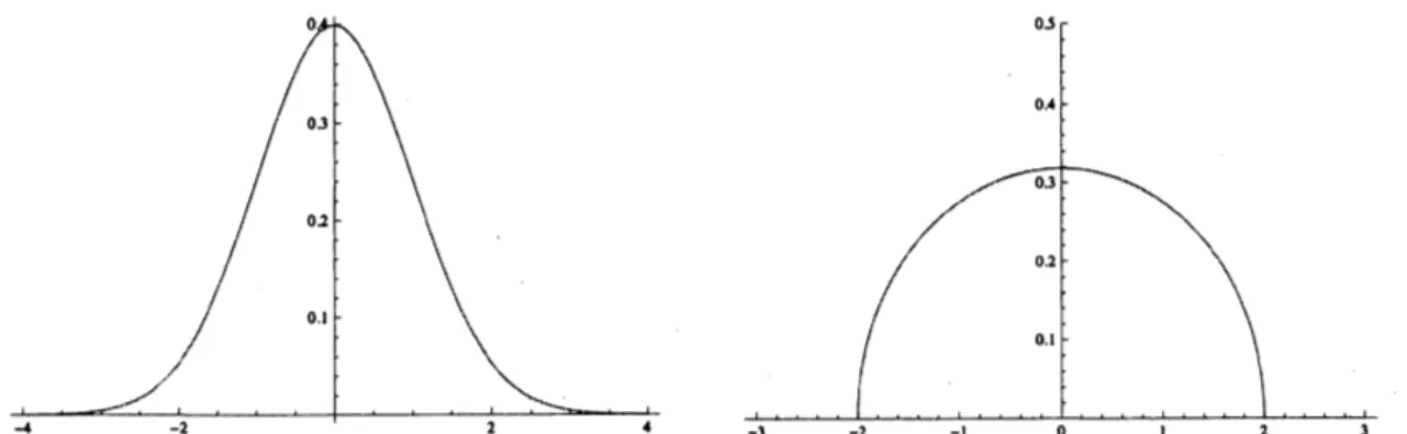
By defining $X_{t}^{(n)}$ _{$:=f_{n}^{X}$}, the situation is the central limit theorem, so the

distri-bution of$X_{1}^{(n)}+\cdots+X_{n}^{(n)}$ converge to _{the standard} Gaussian

$g(dx)=\frac{1}{\sqrt{2\pi}}e^{-\frac{x^{2}}{2}}1_{\mathbb{R}}(x)dx.$

The Gaussian is the most important $ID$ law.

(2) Let $\lambda>0$ be real and $n>\lambda$ be natural numbers. Assume $\mathbb{R}$-valued random

variables $X_{i}^{(n)}$ take $0$ at probability $1- \frac{\lambda}{n}$, and take 1 at probabihty $\frac{\lambda}{n}$, and they are

independent withrespect to $i$ for each _$n$. Then the distribution of$X_{1}^{(n)}+\cdots+X_{n}^{(n)}$

weakly converge to the Poisson

distribution4

$p_{\lambda}=\sum_{n=0}^{\infty}\frac{\lambda^{n}e^{-\lambda}}{n!}\delta_{n}.$

In terms ofconvolution,

$((1- \frac{\lambda}{n})\delta_{0}+\frac{\lambda}{n}\delta_{1})^{*n}arrow p_{\lambda} (narrow\infty)$

.

Hence the Poisson distribution is $ID$ for anyparameter $\lambda>0.$

The above definition emphasizes onthe aspect of the limit theorem, but it coincides

with the usual definition of $ID$ distributions.

Proposition 2.3. $A$ probability

measure

$\mu$ on

$\mathbb{R}$ is $ID$

if

and only

if

for

each $n\in$

$\{1,2,3, \cdots\}$ there exists aprobability

measure

$\mu_{n}$ such that

Every$ID$ distribution appears as the distribution ofa L\’evy process. Thisextends the

fact that the

Gaussian

is the distribution of

a

Brownianmotion. The reader

can

consult

[S99] for L\’evy processes.

Nowwe aregoingtodefineafree version of$ID$distributions. This concept is hopefully

useful for a better understand of free convolution ffl and the

sum

of random matrices.

Definition 2.4 ([BV93]). $A$ probability

measure

$\mu$ on

$\mathbb{R}$ is said to be freely infinitely

divisible $(FID)$ if for any $n\geq 1$ there exist identically distributed, freerandom variables

$X_{1}^{(n)},$

$\cdots,$

$X_{n}^{(n)}$ such that the distribution of$X_{1}^{(n)}+\cdots+X_{n}^{(n)}$ weaMy converge to $\mu.$

Thefree analogueofProposition2.3 isalsothecase. Thisfactwasproved by Bercovici

and Pata[BP99]. Note that a

more

general hmit theorem

was

proved by Chistyakovand

G\"otze [CG08].

Figure 1: Probabihty density of the stan- Figure 2: Probabihty density of Wigner’s

dard Gaussian $g$ semicircle law$w$

Figure4: Probability densityof free Poisson

Figure 3: Poisson distribution $p_{1}$

Example 2.5. (1) Suppose $(X_{i})_{i\geq 1}$ beidenticallydistributed,free random variables and

$\varphi(X_{i})=0,$ $\varphi(X_{i}^{2})=1$. Define $X_{i}^{(n)}$

$:=\pi_{n}^{X}$, then as $narrow\infty$, the distributions of

random variables $X_{1}^{(n)}+\cdots+X_{n}^{(n)}$ weakly converge to Wigner’s semicircle law

$w(dx)=\frac{1}{2\pi}\sqrt{4-x^{2}}dx.$

Therefore Wigner’s semicircle law is FID. This measure appears as the limiting

eigenvaluedistribution of GUE ensemble. This distribution was found by Wigner in

his approach _{to modeling statistics of energy levels of nucleons in nuclei. Recently}

Wigner’s result has been refined by some research groups. Tao and Wu wrote a

summary on this subject [TV].

(2) What should be called the

_free

Poisson distribution is defined as follows:

$\pi_{\lambda}:=\lim_{narrow\infty}((1-\frac{\lambda}{n})\delta_{0}+\frac{\lambda}{n}\delta_{1})^{ffln} \lambda>0.$

When $\lambda=1^{\backslash }$, the probabihty density function of

$\pi_{1}$ can be written as

$\frac{1}{2\pi}\sqrt{\frac{4-x}{x}}1_{[0,4]}(x)dx.$

This distribution is also called the Marchenko-Pastur distribution that is known to

appear

as

the eigenvalue distribution of the square of GUE; one

can

check that if a

random variable $X$ follows $w$, then $X^{2}$ follows

$\pi_{1}.$

Because free convolution is linearized by the Voiculescutransform, it is expectedthat

FID distributions can be characterized by the Voiculescu transform, and it is indeed the

case.

Theorem 2.6 (Bercovici-Voiculescu [BV93]). The following are equivalent.

(1) $\mu$ is $FID.$

$(2)-\phi_{\mu}$ analytically continues to $\mathbb{C}^{+}$ and it maps $\mathbb{C}^{+}$ into $\mathbb{C}^{+}\cup \mathbb{R}^{5}$

(3) Constants $\eta\in \mathbb{R},$$a\geq 0$ and nonnegative

measure

$\nu$ exist satisfying $\nu(\{0\})=0,$

$\int_{\mathbb{R}}\min\{1, x^{2}\}\nu(dx)<\infty$, and

$z \phi_{\mu}(z^{-1})=\eta z+az^{2}+\int_{R}(\frac{1}{1-xz}-1-xz1_{[-1,1]}(x))\nu(dx)$, $z\in i(-\infty, 0)$. $(2.1)$

Theintegral representationin (3) corresponds to theL\’evy-Khintchine representation

in probability theory [S99]. The

measure

$v$ is called the

free

L\’evy measure of

$\mu$

.

In the

classical case, a probabihty

measure

$\mu$ is $ID$ if and only if

$\log\hat{\mu}(z)=\log(\int_{\mathbb{R}}e^{izx}\mu(dx))$

(2.2)

$=i \eta z-\frac{1}{2}az^{2}+\int_{\mathbb{R}}(e^{ixz}-1-ixz1_{[-1,1]}(x))v(dx) , z\in \mathbb{R},$

where $\eta,$$a,$$\nu$ satisfy the

same

conditions as in (2.1). If we replace

$e^{z}$ by $\frac{1}{1-z}$ and then $iz$

by $z$ in (2.2), we obtain (2.1) except the difference of the coefficient of

$z^{2}$

.

Thus the two

representations arequite similar, but theproofsare totallydifferent. Thissimilaritywas

investigated in [BP99] froma viewpoint oflimit theorems. The correspondence between

$\frac{1}{1-z}$ and $e^{z}$

was

discussed in [BT06].

What kind of distributions are FID? In probability theory, a lot of$ID$ distributions

are known and they appear in many applications. There are several sufficient conditions

forameasureto be$ID$

.

Ifa measurehas a probabilitydensityfunction that is completely

monotone or$\log$ convex, then the

measure

is $ID$

.

Note that a function $f$ : $(0, \infty)arrow \mathbb{R}$is

completely monotone ifthere exists a Borel

measure

$\sigma$ such that

$f(x)= \int_{0}^{\infty}e^{-xt}\sigma(dt)$

.

Or if thedensityfunction is HCM (hyperbohccompletelymonotone), the

measure

is $ID.$

The book [SH03] contains the summary of past results,including thesufficient conditions

explained in the above.

By contrast, existing FID distributions with concrete density functions

are

not so

many in free probability, nor useful sufficient conditions. The author’s recent work is

mainly on finding examples of FID distributions, which hopefully leads to sufficient

conditions for a probabihty

measure

to be FID.

3

Research

achievements

on

FID

distributions

3.1

Explicit

probability density

and explicit Voiculescu

trans-form

When $\phi_{\mu}$ is computable, Theorem 2.6(2) is useful to

see

whether $\mu$ is FID

or

not.

Wigner’s semicircle law has the Voiculescutransform $\phi_{w}(z)=\frac{1}{z}$, and the freePoisson law

$h_{\mathfrak{B}}\phi_{\pi_{\lambda}}(z)=\frac{\lambda z}{z-1}$, but there

are

not many examples. Recently, Arizmendi,

Bamdorff-Nielsen and P\’erez-Abreu [ABP10] found that the symmetrized beta distribution with

parameters $\frac{1}{2},$$\frac{3}{2}$

$b_{s}(dx) :=\frac{1}{\pi\sqrt{s}}|x|^{-1/2}(\sqrt{s}-|x|)^{1/2}dx, -\sqrt{s}\leq x\leq\sqrt{s}$

has explicit Stieltjes and Voiculescu transforms:

$G_{b_{s}}(z)=-2^{1/2}( \frac{1-(1-\mathcal{S}(-\frac{1}{z})^{2})^{1/2}}{S}1^{1/2}$

(3.1)

$\phi_{b_{s}}(z)=-(\frac{1-(1-\frac{s}{2}(-\frac{1}{z})^{2})^{2}}{s})^{-1/2}-z.$

We

can see many

powers in (3.1), and so we tryto extend thesepowers followingthe paper [AHb].

Definition 3.1. For $0<\alpha\leq 2,$ _$r>0,$ $\mathcal{S}\in \mathbb{C}\backslash \{0\}$, define the function $G_{s,r}^{\alpha}$ as follows:

$G_{s,r}^{\alpha}(z)=-r^{1/\alpha}( \frac{1-(1-s(-\frac{1}{z})^{\alpha})^{1/r}}{s})^{1/\alpha}$

Also we denote its reciprocal by $F_{s,r}^{\alpha}(z)$ $:= \frac{1}{G_{s,r}^{\alpha}(z)}$

.

It tums out easily that $F_{s,1}^{\alpha}(z)=z.$

The reader probably wonders why such a deformation appears. The reason is

sum-marized in the following relation.

Theorem 3.2 (Arizmendi-Hasebe [AHb]). For $r,$$u>0,2\geq\alpha>0,$ $s\in \mathbb{C}\backslash \{0\}$, we

obtain

$F_{s,r}^{\alpha}\circ F_{us,u}^{\alpha}=F_{us,ur}^{\alpha}.$

In the particular case $u= \frac{1}{r}$, this relation reads $(F_{s,r}^{\alpha})^{-1}=F_{s/r,1/r}^{\alpha}.$

This deformationis considered so that the above relation holds. $A$ remarkable point

is that the inverse function $(F_{s,r}^{\alpha})^{-1}$ is contained in the original family, so that the

com-putation of $\phi_{\mu}$ is possible.

We have deformed the Stieltjes transform of $b_{S}$, but we have to show that the

de-formed family still corresponds toprobability measures.

Theorem 3.3. Let $1\leq r<\infty,$ $0<\alpha\leq 2$

.

Assume one

of

thefollowing conditions:

(i) $0<\alpha\leq 1,$ $(1-\alpha)\pi\leq\arg s\leq\pi$;

(ii) $1<\alpha\leq 2,0\leq\arg s\leq(2-\alpha)\pi.$

Then $G_{s,r}^{\alpha}$ is the Stieltjes

tmnsform of

aprobability

measure

$\mu_{s,r}^{\alpha}.$

The

measures

$\mu_{s,r}^{\alpha}$ contain some well known distributions. When $(\alpha, s, r)=(2, s, 2)$,

the

measure

$\mu_{s,2}^{2}$ is the symmetrized beta $b_{s}$, and when $( \alpha, s, r)=(1, -1, \frac{1}{a})$, the beta

distribution

$\beta_{1-a,1+a}(dx)=\frac{\sin(\pi a)}{\pi a}x^{-a}(1-x)^{a}dx, 0<x<1$

$1aw\pi_{1}$ uptoscaling. $UsingtheexphcitVoicu1$escutransform

$\phi_{\mu_{s,r}^{\alpha}}$ andTheorem2$.6,$

weappears.

$Intheparticularcasea=\frac{1}{2},$ themeasure$\beta_{1/2’ 3/2}coincideswiththefreePoisson$

can prove

the following.

Theorem 3.4. Assume that $(\alpha, s, r)$

satisfies

the assumption

of

Theorem 3.3. Then

(1) $\mu_{s,2}^{\alpha}$ is $FID.$

(2) $\mu_{s,r}^{\alpha}$ is $FID$

if

$0<\alpha\leq 1$ and $1\leq r\leq 2.$

(3) $\mu_{s,r}^{\alpha}$ is $FID$

if

$1\leq\alpha\leq 2$ and $1 \leq r\leq\frac{2}{\alpha}.$

(4) $\mu_{s,3}^{1}$ is $FID$

if

and only

if

_$s$ is purely imaginary.

(5)

_If

$\alpha>1$, there exists _{$r_{0}=r_{0}(\alpha, s)>1$ such that}

3.2

Explicit

probability

density

but

implicit

Voiculescu

trans-form

Recent work has found many other examples of FID distributions. In most cases, the

Voiculescu transform $\phi_{\mu}$ cannot be expressed exphcitly,

so

that the proofs become

more

techmical.

Theorem 3.5. The following probability distributions

are

$FID.$

(1) (Belinschi et al. [BBLSl$1J$) The Gaussian

$g(dx)=\frac{1}{\sqrt{2\pi}}e^{-\frac{x^{2}}{2}}1_{R}(x)dx.$

(2) (Anshelevich et al. [ABBLIOJ) The $q$

-Gaussian

distribution

$g_{q}(d_{X})=\frac{\sqrt{1-q}}{\pi}\sin\theta(x)\prod_{n=1}^{\infty}(1-q^{n})|1-q^{n}e^{2i\theta(x)}|^{2}1[-\frac{2}{\sqrt{}1-q},\frac{2}{\sqrt{}1-q}]^{(x)d_{X}}$

for

$q\in[O, 1)$, where$\theta(x)$ is the solution$ofx= \frac{2}{\sqrt{1-q}}\cos\theta,$ $\theta\in[0,\pi]$

.

When$qarrow 1,$ $g_{q}$

converges weakly to $g$, and $g_{0}$ coincides with $w$

.

For$q\in(O, 1)$, the density

function

of

$g_{q}$

can

be written as $[LM95J$

$\frac{1}{2\pi}q^{-\frac{1}{8}}(1-q)^{\frac{1}{2}}\Theta_{1}(\frac{\theta(x)}{\pi}, \frac{1}{2\pi i}\log q)$ ,

where $\Theta_{1}(z, \tau);=2\sum_{n=0}^{\infty}(-1)^{n}(e^{i\pi\tau})^{(n+\frac{1}{2})^{2}}\sin(2n+1)\pi z$ is a Jacobi theta

function.

(3) ($A$rtzmendi-Belinschi _$[ABJ)$ The ultraspherical distribution

$\frac{1}{16^{n}B(n+\frac{1}{2},n+\frac{1}{2})}(4-x^{2})^{n-\frac{1}{2}}1_{[-2,2]}(x)dx$

for

$n=1,2,3,$$\cdots.$

(4) (Arizmendi-Hasebe-Sakuma [AHSJ) Let $X$ be a mndom variable foltowing Wigner’s

semicircle law. Then $X^{4}$ also

follows

a $FID$ law.

(5) (Arizmendi-Hasebe-Sakuma [AHSJ) The chi-square distribution

$\frac{1}{\sqrt{\pi x}}e^{-x}1_{[0,\infty)}(x)dx.$

(6) (Arizmendi-Hasebe $[AHaJ)$ The Boolean stable law $b_{\alpha}^{\rho}$ is

defined

by

(i) $F_{b_{\alpha}^{\rho}}(z)=z+e^{i\pi\rho\alpha}z^{-\alpha+1}$

for

$\alpha\in(0,1)$ and $\rho\in[0,1]$;

(ii) $F_{b_{\alpha}^{\rho}}(z)=z+2 \dot{\mu}-\frac{2(2\rho-1)}{\pi}\log z$

for

$\alpha=1$ and$\rho\in[0,1]$;

$b_{\alpha}^{\rho}$ is $FID$

if

and only

if.

$\cdot$

$(a)0< \alpha\leq\frac{1}{2}$ and $\rho\in[0,1];(b)\frac{1}{2}\leq\alpha\leq\frac{2}{3}$ and

$2- \frac{1}{\alpha}\leq\rho\leq\frac{1}{\alpha}-1;(c)\alpha=1$ and $\rho=\frac{1}{2}$. For$\alpha<1$, theprobability density

function

can

be written in the

_form

$\frac{db_{\alpha}^{\rho}}{dx}=\{\begin{array}{ll}\sin(\pi\rho\alpha) \pi \frac{x^{\alpha-1}}{x^{2\alpha}+2x^{\alpha}\cos(\pi\rho\alpha)+1}, x>0,\sin(\pi(1-\rho)\alpha) \pi \end{array}$

$\frac{|x|^{\alpha-1}}{|x|^{2\alpha}+2|x|^{\alpha}\cos(\pi(1-\rho)\alpha)+1},$ $x<0,$

(7) $(Bo\dot{z}ejko$-Hasebe $[BHJ)$ The Meixner distribution

$\frac{4^{t}}{2\pi\Gamma(2t)}|\Gamma(t+ix)|^{2}1_{\mathbb{R}}(x)dx$

for

$0<t \leq\frac{1}{2}.$

(8) $(Bo\dot{z}ejko$-Hasebe _$[BHJ)$ The logistic distribution

$\frac{\pi}{2}(\frac{1}{\cosh\pi x})^{2}1_{\mathbb{R}}(x)dx.$

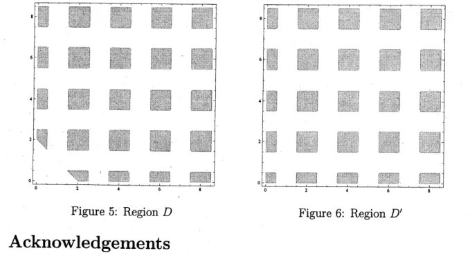
(9) (Hasebe $[HJ)$ The beta distribution

$\sqrt{}p,q(dx)=\frac{1}{B(p,q)}x^{p-1}(1-x)^{q-1}1_{[0,1]}(x)dx$

for

$(p, q)\in D$

.

The _region $D$ is shown in Fig. 5. This result extends (3).

(10) (Hasebe $[HJ)$ The beta prime distribution

$\frac{1x^{p-1}}{B(p,q)(1+x)^{p+q}}1_{[0,\infty)}(x)dx$

for

$(p, q)\in D’$

.

The _region $D’$ is shown in Fig. 6.

(11) (Hasebe $[HJ)$ The $t$-distribution

$\frac{11}{B(\frac{1}{2},q-\frac{1}{2})(1+x^{2})^{q}}1_{\mathbb{R}}(x)dx$

for

$q \in(\frac{1}{2},2]\cup[2+\frac{1}{4},4]\cup[4+\frac{1}{4},6]\cup\cdots$

(12) (Hasebe $[HJ)$ The gamma distribution

$\frac{1}{\Gamma(p)}x^{p-1}e^{-x}1_{[0,\infty)}(x)dx$

(13) (Hasebe $[HJ)$ The inverse gamma distribution

$\frac{1}{\Gamma(p)}x^{-p-1}e^{-1/x}1_{[0,\infty)}(x)dx$

for

$p_{-} \in(0, \frac{1}{2}]\cup[\frac{3}{2}, \frac{5}{2}]\cup[\frac{7}{2}, \frac{9}{2}]\cup\cdots.$

Remark 3.6. We mention

some

remarks on the above results.

(4) It is not known whether $|X|^{q}(q\in \mathbb{R})$ is FID

or

not, except $q=2,4$

.

For $q=2,$ $X^{2}$

follows the free Poisson law $\pi_{1}$ which is FID.

(6) The Boolean stable law is characterized by

some

stability, but not with respect to

classical convolution, but Boolean convolution which appears as the sum of Boolean

independent random variables [SW97].

(7) The Meixner distributions $($for $t>0)$

are

laws of a L\’evy process, called

a

Meixner

process [ST98], since theyhavethe characteristic functions $( \frac{1}{\cosh(z/2)})^{2t}$ When$t= \frac{1}{2},$

the Meixner distribution coincides,with

$\frac{1}{\cosh\pi x}1_{\mathbb{R}}(x)dx,$

which is called the hyperbohc secant distribution. It is known

as

the law ofL\’evy’s

stochastic area [L51].

It is unknown whether the Meixner distributions are FID for $t> \frac{1}{2}$ or not.

(9,10) The beta distributions contain the affine transformations of Wigner’s semicircle law

and the free Poisson law. The beta prime distributions contain the affine

transfor-mation of a free $\frac{1}{2}$-stable law [BP99].

Some parameters $(p, q)$ outside the regions $D,$ $D’$ correspond to

non

FID

distribu-tions, but some still remain to be unknown whether they are FID or not.

(12,13) The gamma distributions and inverse gamma distributions are limits of beta and

prime beta distributions,

so

that they

are

FID as consequences of Theorem 3.5(9),

(10). The result (12) extends (5).

The probability measures above are $ID$ too except (3), (4), (9) and part of (6) The

proofs can be found in Bondesson’s bo$ok$ [B92].

In the same book, the class of GGCs (generalized gamma convolutions) is studied

in details

as

a subclass of $ID$ distributions. The main tool in the analysis of GGCs is

Pick-Nevanlinnafunctions, the same tool

as

used in free probability. The author is now

focusing

on

this similarity in two probabilities and hoping to discover

a

general theory

behind them.

$6The$ _{Boolean stable law is} $ID$when positive, i.e. $\rho=1$. If$\rho\neq 1$, the author doesnot know ifthe

Figure 5: Region $D$ Figure 6: Region $D’$

Acknowledgements

This work was supported by Global $COE$ Program at Kyoto University.

References

[ABBL10] M. Anshelevich, S.T. Behnschi, M. Bozejko and F. Lehner, $\mathbb{R}ee$ infinite divisibility

for $Q$-Gaussians, Math. Res. Lett. 17 (2010), 905-916.

[ABP10] _{O. Arizmendi, O.E. Barndorff-Nielsen andV. P\’erez-Abreu, On freeandclassicaltype}

G distributions, Braz. J. Probab. Stat. 24, No. 2 (2010), 106-127.

[AB] O. Arizmendi and S.T. Belinschi, Free infinite divisibility for ultrasphericals, Infin.

Di-mens. Anal. Quantum Probab. Relat. Top., to appear. arXiv:1205.7258

[AHa] O. Arizmendi and T. Hasebe, Classical and free infinite divisibility for Boolean stable

laws, _{Proc. Amer. Math. Soc., to appear. arXiv:1205.1575}

[AHb] O. Arizmendi and T. Hasebe, Onaclass of exphcit _{Cauchy-Stieltjes transforms related}

to monotone stable and free Poisson laws, Bernoulli, to appear. arXiv:1108.3438

[AHS] _{O. Arizmendi, T. Hasebe and N. Sakuma, On the law of free subordinators.}

arXiv:1201.0311

[BT06] 0.E. Bamdorff-Nielsen and S. Thorbjmsen, Classical andfree infinite divisibilityand

L\’evy processes, In: Quantum Independent Increment Processes II, M. Sch\"urmann and

U. Franz (eds), Lecture Notes in Math. 1866, Springer, Berlin, 2006.

[BBLSII] S.T. Behnschi, M. Bozejko, F. Lehner and R. Speicher, The normal distribution is

ffl-infinitelydivisible, Adv. Math. 226, No. 4 (2011), 3677-3698.

[B09] F. Benaych-Georges, Rectangularrandom matrices,relatedconvolution, Probab. Theory

Relat. Fields 144 (2009), 471-515.

[BP99] H. Bercovici and V. Pata, Stable laws and domains of attraction in free probability

theory (with an appendix by Phihppe Biane), Ann. of Math. (2) 149, No. 3 (1999),

1023-1060.

[BV93] H. Bercoviciand D. Voiculescu, $\mathbb{R}ee$convolution ofmeasureswith unbounded

support,

[B92] L. Bondesson, Generalized gamma convolutions and related classes ofdistributions and

densities, Lecture Notes in Stat. 76, Springer, New York, 1992.

[BH] M.Bozejko and T.Hasebe, On free infinitedivisibilityforclassical Meixner distributions.

arXiv:1302.4885

[CG08] B.P. Chistyakov and F. G\"otze, Limit theorems in free probability theory I, Ann.

Probab. 36, No. 1 (2008), 54-90.

[H] T. Hasebe, in preparation.

[HPOO] F. Hiai and D. Petz, The Semicircle Law, Free Random Variables andEntropy.

Math-ematical Surveys and Monographs Vol. 77, Amer. Math. Soc., 2000.

[LM95] H. van Leeuwen and H. Maassen, A$q$-deformation oftheGauss distribution, J. Matb.

Phys. 36 (1995), No. 9, 4743-4756.

[L] R. Lenczewski, Limit distributions of random matrices. arXiv:1208.3586

[L51] P. L\’evy, Wiener’s randomfunctions, and other Laplacian random functions, Proc. 2nd

BerkeleySymp. on Math. Statist. and Prob. (Univ. ofCalifomiaPress, 1951), 171-187.

[M04] M.L. Mehta, Random matrices, Amsterdam, Elsevier/Academic Press, 2004.

[M03] N. Muraki, The fiveindependences as natural products, Infin. Dimens. Anal. Quantum

Probab. Relat. Top. 6, No. 3 (2003), 337-371.

[S99] K. Sato, L\’evy Processes and Infinitely Divisible Distributions, Cambridge University

Press, Cambridge, 1999.

[ST98] W. Schoutens and J.L. Teugels, L\’evy processes, polynomials and Martingales,

Com-mun. Statist.-Stoch. Mod. 14 (1998) 335-349.

[SW97] R. Speicher and R. Woroudi, Boolean convolution, in Free Probability Theory,

Ed.

D.

Voiculescu, Fields Inst. Commun., vol. 12 (Amer. Math. Soc., 1997), 267-280.

[SH03] F.W. Steutel and K. VanHarn,

_Infinite

Divisibility

_of

Probability Distributions on the

Real Line. Marcel-Dekker, New York, 2003.

[TV] T. Tao and V. Vu, Random matrices: The universality phenomenon for Wigner

ensem-bles. arXiv:1202.006S

[V85] D. Voiculescu, Symmetries of some reduced free product algebras, Operator algebras

and their connections with topology and ergodic theory, Lect. Notes in Math. 1132,

Springer, Berlin (1985), 556-588.

[V86] D. Voiculescu, Addition of certain non-commutative random variables, J. Funct. Anal.

66 (1986), 323-346.

[V91] D. Voiculescu, Limit laws for random matrices and free products, Invent. Math. 104,

No. 1 (1991), 201-220.

[VDN92] D. Voiculescu, K.J. Dykema and A.M. Nica, Foee Random Variables, CRM

Mono-graph Series, Vol. 1, Amer. Math. Soc., Providence, RI, _1992.

[W86] W. Woess, Nearest neighbour random walks on free $pr\sigma$ducts of discrete groups,