Program Evaluation : Education and
Health Expenditure of Households in
Indonesia
Herbert Agust Suranta Munthe
Department of Taxes, Ministry of Finance, Indonesia
*Kazuo Inaba
Faculty of Economics, Ritsumeikan University
Contents1.Introduction
2.The Program, Education and Health Issue in Indonesia 3.Theoretical Framework
4.Data and Methodology 5.Empirical Analysis
6.Conclusion and Policy Implication
Abstract
This paper intends to investigate whether the program affects the expenditure of households in Indonesia, especially with respect to education and health expenditure. Using the cross-sectional data from the Indonesia Family Life Survey 4 and employing the propensity score matching method and the two stage least square method, the study finds that the program affects education expenditures, whereas there is no evidence that the program affects health expenditures of beneficiaries.
The study also investigates the household and demographic characteristics as determinants of education and health expenditures. The paper finds that, in general, household and demographic characteristics play a significant role in education and health expenditures.
Based on the estimated results the paper suggests that the government should keep implementing the program with some points. First, the government and Non-Government Organization (NGO) should enhance and monitor the targeting program. Second, the government could provide some programs that generate and create income, such as workplace, loans, or health insurance to the poor households. In addition, in order to avoid becoming a burden that the government supports, the government should sustain economic
growth that can create employment and better income to skillful and healthy workers. Key words : Raskin program, poverty alleviation, propensity score matching method, the
two stage least square (2SLS)
1
.Introduction
Many developing countries have implemented various programs to alleviate poverty. Usually the programs involved developed countries or international agencies such as the International Monetary Fund (IMF), the World Bank (WB), the Asian Development Bank (ADB), and many more as fund sponsors. Yet, not all these efforts have fulfilled
expectations. As a result, income inequality remains high.
The government of Indonesia had one famous program implemented for poor people called (Rice for the Poor). This program was implemented for more than ten years, since the Asian Financial crisis affected the Indonesian economy in 1998. The main aim of the program was to support food for the needy households. It was expected that the program would be able to decrease income inequality.
The program provided subsidized rice at price 1,000 rupiah1) per kilogram for each beneficiary. All beneficiaries were supposed to receive 20 kilogram of subsidized rice every month for one year. From 1998 until 2007, the price paid by beneficiaries was fixed ; therefore, the main purpose of the program was food adequacy first, but also aided income transfer as well. In other words, this program became a combination of income transfer and food adequacy aid. Therefore, it is interesting to know how participants allocate their additional income to certain expenditures.
Meanwhile, the previous studies suggested that education and health played a big role in human development quality. They suggested that better education and health lead to a better economic life (Card, 1999 ; Tilak, 2002). This means that a better level of education and health will secure better jobs and income and in the end raise the economic status of the individual.
The United Nation Development (UNDP) stated that the expected and mean years of schooling in Indonesia were increasing slightly from 1980 to 2006. In addition, the literacy rate above 10 years old increased from 61 percent in 1971 to 93 percent in 20072).
Accordingly, the Central Statistics Bureau (BPS) stated that from 2000 until 2007 the nominal and the percentage share of education expenditures either in urban or rural areas had a trend towards increasing. We discovered a similar trend to the nominal and the percentage share of the health expenditures in both areas3).
The information above suggests that the enrolled students and the increased health indicator indicated that the households needed more money to pay for both expenditures. In other words, the expenditures on education and health should have increased as the children could afford higher levels of education and health.
induced the participants of the program to change their share of expenditure on education and health by using propensity score matching (PSM) and the two stage least square (2SLS) method.
The remainder of this study is structured as follows : Section 2 provides information on the program, the education and health in Indonesia. Section 3 presents the theoretical and reviews of some selected empirical literatures. Section 4 procures the data and methodology applied in this study. Section 5 is empirical analysis and discussion. The final section is the conclusion with some policy implications
2
.The
Program, Education and Health Issue in Indonesia
2―1 An Overview of the Program
( ) literally meaning rice for the poor, was a
program by the Indonesian Government that intended to reduce the financial burden of poor households and to maintain the improvement of food adequacy needed by providing subsidized rice.
This targeted program was a transformation of the Special Market Operation, (Operasi Pasar Khusus / OPK), which was part of the Social Safety Net (SSN) when the Asian Financial Crisis hit Indonesia in 1998. A poor household definition used in OPK program was based on classification introduced by the National Family Planning Board (Badan Kesejahteraan Keluarga Berencana Nasional / BKKBN). They were
(pre-prosperous), (prosperous level I) which is almost poor, KS
III and KS IV. The beneficiaries of the program were households in the first two classifications. The village official had the list of the beneficiaries based on this classification, i. e., the first two classifications, where the households bought the rice from the National Logistic Agency (the BULOG). Then all beneficiaries bought the rice from the village official at a price of 1,000 rupiah plus some amount of additional transportation cost. Hastuti (2007) found that there were some weaknesses in targeting the beneficiaries and implementation of the OPK program. They revealed that measuring the poverty based on the consumption had less correlation with classification of poor households introduced by the BKKBN. Therefore, the program had underestimated the targeted households by a significant number. The poor households classifications were mainly for the contraceptive user purpose. In addition, the classification was updated only once a year, so the dynamics of the households conditions could not be recorded. Most importantly, the classification was based on the static criteria such as having clothes and housing conditions rather than the current welfare situation.
Under these conditions, the government transformed the OPK program into rice for the poor family, with some adjustments such as the concept, the implementation, and the source of the data to target the beneficiaries, distribution frequency, and designation of the institution assisting the local agents.
2―2 The Beneficiaries of the Program
After transforming the program from OPK to the method of targeting changed drastically. The beneficiaries of the program were poor households classified into very poor and poor. These poor households were selected by referring to data from SUSENAS 2005 (National Socio-Economic Survey) conducted by the BPS. The BPS measures poverty by using basic needs consumption fulfillment. The poverty threshold referred to the total value of food expenditures to afford a daily minimum of 2,100 kilocalories and non-food expenditures such as clothing, schooling, transportation and other individual basic needs reported by families. Those families with per capita expenditures below this poverty line are categorized as poor. All of these poor families were supposed to participate in the program. In fact, the implementation was weak because the program did not cover all of them.
Furthermore, the government relaxed the rule that provided a possibility for a family categorized as almost poor to become a beneficiary. Through the village forum decision (musyawarah desa / ), the village head decided which of these poor and almost poor households were to become participants. Once a year before the rice distributed, the village forum arranged a meeting. This meeting resulted in the list of beneficiaries of each village. The sub-district head approved the result and forwarded the final list to the higher levels until reached the province level. The BULOG, who was in charge of supplying the rice, referred to the list in distributing the rice until the local distribution point at the price of 1,000 rupiah per kilogram. Moreover, the beneficiaries should pay for the rice in cash to the local distribution agent directly or transmit the money to the BULOG s account before receiving the rice4). This became one of the weaknesses of the program since not all poor households had cash.
The government implemented this program based on the households condition and characteristics with no differentiation between regional poverty conditions. This was because the poor households were spread evenly throughout all regions.
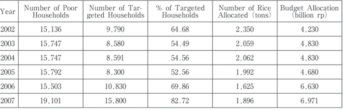
Table. 1 shows that the number of targeted households was increasing year by year, but still below the total poor households based on the SUSENAS data. Contrary to that, the amount of rice allocated decreased from 2.34 tons to 1.89 tons. This was because the
Table 1. The Number of Targeted Households and the Amount of Rice Distributed (thousands) Year Number of Poor Households geted HouseholdsNumber of Tar- % of Targeted Households Allocated (tons)Number of Rice Budget Allocation (billion rp)
2002 15,136 9,790 64.68 2,350 4,230 2003 15,747 8,580 54.49 2,059 4,830 2004 15,747 8,591 54.56 2,062 4,830 2005 15,792 8,300 52.56 1,992 4,680 2006 15,503 10,830 69.86 1,625 6,630 2007 19,101 15,800 82.72 1,896 6,971 Source : BULOG
government reduced the amount of rice distributed from 20 kg per month in 2005 to only 10 kg in 2006.
Moreover, the purchase price in 2007 was 4,616 rupiah per kilogram. This indicated that the government allocated the subsidy around 3,616 rupiah per kilogram5). In addition, the subsidized price of the rice included the transportation cost up to the point of distribution and other administration fees such as official bonuses and honorariums. Therefore, the beneficiaries did not need to pay any additional money to get the rice.
2―3 Education Issue in Indonesia
There are three basic level of education in Indonesia : elementary, junior, and senior high level. The advanced level is college, while playgroup or kindergarten is not a compulsory. The length of time spent at the elementary level is six years, whereas for each of the junior or senior level is three years. The usual age for a child to begin elementary school is seven years old.
Indonesia started a nine-year compulsory education in 19946). The government provides facilities such as public schools and rules related to school administration while the households utilize those facilities.
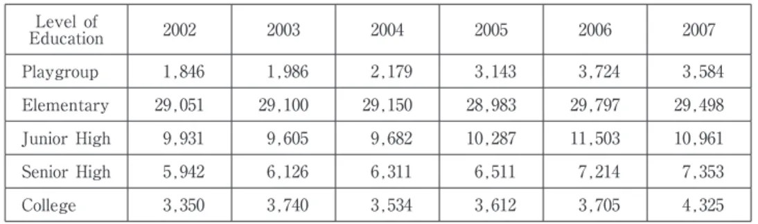
Table 2 shows the number of enrolled students for each level of education from 2002 to 2007 in Indonesia. The elementary level still dominates the composition of schoolchildren. For each year, the number of enrollment at the junior level was half of the total elementary children. This indicated that the rate of students dropping out or the amount of students that could not afford the higher level was significant. It was similar to other higher levels of education where the enrolled students decreased by almost half as the level of education increased.
Furthermore, the number of enrolled students tended to increase from year to year for all levels of education. On the other hand, the enrolled students at the elementary and junior level tend to decline compared to the previous year.
2―4 Health Development in Indonesia
In 1999, Law Number 22 on Regional Government was enacted. This law was revised in 2004 through Law Number 32. This law ruled the government system from centralized to
Table 2. The Enrollment Students by Level of Education (thousands) Level of Education 2002 2003 2004 2005 2006 2007 Playgroup 1,846 1,986 2,179 3,143 3,724 3,584 Elementary 29,051 29,100 29,150 28,983 29,797 29,498 Junior High 9,931 9,605 9,682 10,287 11,503 10,961 Senior High 5,942 6,126 6,311 6,511 7,214 7,353 College 3,350 3,740 3,534 3,612 3,705 4,325
regional autonomy at the district or municipality level. The law gave the provincial government more authority to manage local affairs except for national defense, monetary and fiscal matters, religion, foreign affairs, and justice.
Following the law, the Ministry of Health stipulated that the goal of health programs and development after Health Law Number 23/1992 was enacted. This law became the basis of health department to provide public health services and activities at the local government level.
The Indonesia Demographic and Health Survey in 2007 revealed that most of Indonesian people cited income as the main barrier to receiving better health service or treatment. This barrier was followed by distance to public health care, transportation, and unemployed spouse. Therefore, the Indonesian government provided affordable health services through some health programs for the poor such as Social Security for the Poor, Health Fund, and Poor Health Card ( ). Even though there are many pro poor programs in the health sector, studies revealed that the private spending on health still dominated health expenditures in Indonesia.
Moreover, Figure 1 explains that the government only spent 36.6 percent of total health expenditures, whereas the private share was 63.4 percent. From the 63.4 percent of private expenditure, 76.1 percent was out of pocket, while 5.1 percent was pre-paid and the rest was from other sources. This indicates that households still have to share more of their income on health expenditures7).
3
.Theoretical Framework
Sumarto, Suryahadi and Widiyanti (2004) suggested that this program has become a combination of income transfer and food adequacy aid because the price of subsidized rice was always constant and the amount was still below the total consumption. In order to
Figure 1. The Share of Public and Private Health Expenditure
Source : BPS OOP 76.1% Private 63.4% Public 36.6% Pre-paid 5.1% Others 18.8%
investigate the program contribution to the expenditure of households, we treat the program as additional income of the beneficiaries.
The utility function of a household s expenditure in Figure 2 explains that by assuming the education and health expenditure are normal goods, a beneficiary would increase their expenditure on both goods if they benefit from the program. The beneficiary takes this action in order to receive the same level of utility maximization. Therefore, the utility maximization shifts from 1 to 2 when there is additional income.
3―1 Conceptual Framework and the Empirical Model
Parents invest in education and health because these two factors are so important for a child s future economic capabilities. Many studies are concerned about the determinants of household education and health. The household production model introduced by Becker (as cited in Sackey, 2007) has been improved and often used to analyze the determinants of human capital building of households. The function is dependent on households and community characteristics. The household production function implies that parents may maximize their resources in order to produce the highest quality of their children. This maximization is obtained through the combination of time and goods.
One main determinant of education and health expenditure is household income. The International Labor Organization defines household income as the total income, whether any member of the household annually or regularly receives income in cash, in kind, or in services. The income does not include the gains from windfalls and other irregular or a one-time receipt. Ordinarily the household income is for current consumption, which does not decrease the value of the household s net worth or all the disposal of the household s financial or non-financial assets, nor does it increase the liabilities of the household.
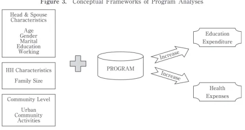
Chen (1990), Rossi, Freeman and Lipsey (1999), and Donaldson (2001) suggested that the theoretical and conceptual approach should be modified with the households and socio demographic characteristics as control variables to analyze a program s impact (Figure 3).
Figure 2. The Effect of Changes in Income
X Income Consumption Curve
Y
U2
B A
Therefore, the empirical household production function has to be modified with program evaluation to examine the outcome estimation, which is given by :
Outcome=(Y, C)
where Y is income of a household and C is a set of household and demographic characteristics. Considering that the program is additional income to the participants, we do not use income as an independent variable instead of the program itself.
The set of characteristics includes the age of the family s head and family size. We also include some dummy variables such as gender, marital status and working status of the household s head, level of education in both the head and spouse of the household (Card, 1999 ; Tansel, 1998 ; Tilak, 2002 ; Thomas, 1994 ; Parker, Susan, and Wong, 1997). Urban as a demographic dummy variable is also included in this study.
3―2 Literature Reviews
Following the theoretical framework above, many studies have analyzed how a program is treated as additional income, which affects the consumption of beneficiaries. Those programs were provided either in cash or in kind transfer.
Houdinott and Skoufias (2003) analyzed how Progresa in Mexico, a targeted program to the mother of families from November 1998 to November 1999, affected the food consumption of participants. This program provided both cash and in kind transfer. The former transfer linked to children s enrollment and school attendance, while the latter included health benefits such as nutrition for children, pregnant women, and lactating women. The study exploited longitudinal data (ENCEL) of 24,000 households located in 506 localities of seven states. Three hundred and twenty of the localities are designated as treatment and the rest are as control communities.
By a fixed effect of OLS method, the paper analyzed the impact of the program on caloric acquisition. The method also used some dummy variables to specify households
Figure 3. Conceptual Frameworks of Program Analyses
Education Expenditure Increase PROGRAM Health Expenses Increase
Head & Spouse Characteristics Age Gender Marital Education Working HH Characteristics Family Size Community Level Urban Community Activities
located in treatment or control localities and participants or non-participants. The result showed an increasing magnitude in the acquisition of fruits and vegetables consumption compare to grains and other food types. Further analysis is observed by including the eligible households that did not receive any transfer due to some reasons. Even though the results are significant, they are still lower than the first observation. Most importantly, the program encourages the beneficiaries to consume a varied diet such as fruits, animal product, milk, and others. Overall, this study suggests that efforts to reduce poverty in the developing world will also reduce hunger.
Attanasio and Menard (2006) analyzed the impact of on
household consumption and its components in Colombia. The three main components of this program are health, education, and nutrition. This targeted program designated the poorest 20 percent of households in selected areas of Colombia.
The program gave beneficiaries a nutrition component worth 40,000 pesos (around US$15) if a household had children aged 0 to 5. In addition, a mother also would receive 14,000 pesos (US$5.5) and 28,000 pesos (US$11) if their children were enrolled and regularly attending primary or secondary school. Not all households received the benefit regularly.
The randomized assignment program used quasi-experimental approach with a difference in difference method. A repeated survey before the program in 2002 and after the program in 2003 made this method applicable. Twenty-five stratified control groups determined by region and index relating to health and education were constructed. As a result, the treatment group consisted of 57 municipalities while counterpart group consisted of 65 municipalities. Due to political pressure, one of the groups had already received the program before the survey data were collected. Following this condition, the treatment group became two groups.
The study argued that the total consumption increased around 15 percent as much as the food consumption. In particular, the increasing share of food consumption was concentrated in proteins such as milk, egg, and meat. In addition, the share of children s clothing and education also increased, but not for adult goods such as alcohol, tobacco, and adult clothing.
Another study on Latin countries is (RPS) in Nicaragua. The Nicaraguan RPS is a program that pays households cash stipends in exchange for school attendance and regular visits to health clinics by the children. Mallucio and Flores (2005) analyzed the heterogeneous impacts of the program on the poor people in Nicaragua. The advantage of this study is that the program was designated randomly. Therefore, the experimental study with a double difference method is perfectly applied. After constructing the control and treatment areas, the average treatment in both groups can be estimated. The study suggested that the program has a large effect on the children s schooling compare to the control group. Another finding of this study found that there was no evidence altering the impact of RPS on school enrollment. Indeed, the program had a significant impact on household food and education expenditure. This impact was primarily
attributable to the income effects.
On average, RPS supplemented total annual per capita household expenditures by 18 percent and most of this increase was spent on food. The program resulted in an average increase of 640 Nicaraguan in annual per capita food expenditures and an improvement in the diet of beneficiary households. Expenditures on education also increased significantly, though there was no discernible effect on other types of investment expenditures. The economic crisis experienced by these communities during the period enabled RPS to operate somewhat like a traditional social safety net, aiding households during a downturn.
4
.Data and Methodology
4―1 Data
Our data sources are primarily from the website of the Rand Corporation. This institution has conducted surveys four times : in 1993, 1997, 2000, and 2007. The repeated longitudinal survey is a socioeconomic and health survey that is called the Indonesia Family Life Survey (IFLS8)).
The Indonesia Family Life Survey was designed to provide data for studying behaviors and outcomes. The survey contains information on wealth collected at the individual and household levels and includes multiple indicators of economic and non-economic well-being such as consumption, income, assets, education, migration, labor market outcomes, marriage, fertility, contraceptive use, health status, use of health care and health insurance, relationships among co-resident and non-resident family members, processes underlying household decision-making, transfers among family members, and participation in community activities.
In addition to individual and household-level information, IFLS provides detailed information on the communities in which IFLS households are located, and the facilities that serve residents of those communities. These data cover aspects of the physical and social environment, infrastructure, employment opportunities, food prices, access to health and educational facilities, and the quality and prices of services available at those facilities The Indonesia Family Life Survey is a continuing longitudinal socioeconomic and health survey. The survey based on a sample of households that represents about 83% of the Indonesian population living in 13 out of the nation s 26 provinces in 1993. The survey collected data on individual respondents in the households, the communities in which they live, and the health and education facilities they use. The first wave (IFLS1), in 1993, administers individuals of 7,224 households. IFLS2 sought to re-interview the same respondents four years later. The next waves were fielded in 2000 (IFLS3) and 2007 (IFLS4). In IFLS4, the numerators tried to re-interview all target households plus households that has been moving or new split-off households that contained at least one target respondent. Finally, the number of households increased, becoming 15,145
households and 66,835 individuals.
Considering the dynamics of the households during the period from 2000 to 2007, we decided to analyze the program only in one year of cross-sectional data, which is in 2007 i. e., IFLS 4. We cannot capture the dynamics of the households, such as separated or newly married household members, death, birth, children starting to school, graduating or dropping out of school, and many more.
The questionnaires about the program are mostly covered in Book I (KSR-code). Table 3 summarizes only IFLS4 data about the number of households that answered the program questions. Among 11,092 households that answered the questions, 43.7% or 4,842 households of them participated, while 56.4% or 6,251 households never participated.
Hastuti and Maxwel (2003) suggested that a subjective decision may occur since the final decision of beneficiaries was determined by the local government and local community meeting ( ). They argue that the lack of transparency was available in determining the participants. We excluded households below the poverty line that did not receive the program, but included households above the poverty line that received the program. We took this action because the number of sample households below the poverty line in the treatment was so small9). If we excluded ineligible households in this group, the estimation results might be not accurate. However, the inclusion of these households may cause a self-selection bias as Heckman, Ichimura, and Todd (1998a ; 1998b) and Bryson, Dorsett, and Purdon (2002) suggested.
In selecting the sample-size for the children s education expenditure, we excluded households that did not have children in school age from 7 to 24 years old and outliers based on per capita expenditure and education expenditure. In terms of health expenditure outcome, we excluded the outliers in per capita health expenditure10). On the other hand, we included all children living in and out of the households that received education expenditures from the family.
We grouped the respondents according to whether they received the program in 2007 or not. Households that received the program are referred to as the treated, whereas those who were not exposed to the program are referred to as the non-treated. All these selections leave us with 661 households as treated and 1,309 households as the non-treated in education outcome, while for health expenditure outcome there are 4,838 households and 1,591 households in the non-treated and the treated, respectively (Appendix A and B).
Table 3. The distribution of respondents
Program Total Respondent
Number %
Non-Participant 6,251 56.35
Participant 4,482 43.65
4―2 Methodology and Data Analysis
The assignment of the program was purposively determined. Thus, the possibility of bias may occur if the treatment has no effect, but the outcomes between two comparison groups are different because they were not comparable before the treatment applied. This potential bias occurs since we only utilize one year s data set.
4―2―1 Propensity Score Matching
Rossenbaum and Rubin (1983) introduced a method to overcome this problem. They propose a method called propensity score matching (PSM) in order to build a comparison group if we do not have the baseline data set.
Figure 4 explains how to analyze a program impact on the participant if we do not have the baseline data. We may obtain the treatment effect of an individual who participates in the program by subtracting the outcome of that individual after the program to his outcome when he does not participate. Rubin (1974) states the treatment effect of this individual as follows :
τi=Y(1)−Yi (0) i ⑴
where τ is the effect of the program, Y is the outcome with Ti equals one if he participates
and zero otherwise. So, the potential outcomes of each individual is Y(T).i
A problem arose because we do not have the baseline data of each individual. Therefore, it is impossible to measure the outcome of the same person after the program at the same time. In other words, it is impossible to obtain an outcome of the individual by comparing it to his own outcome in the post program. The only choice we have is to measure the outcome of all participants. This is what Rubin (1974) calls as the Average Treatment on the Treated (ATT).
Rubin defines the model of the ATT as follows;
Figure 4. Program Impact Analyses
During Program Before Program Pre-Program outcome level
Post-Program outcome level
O ut co m e C ha ng e
τATT=Ε(Y1−Y0 ¦ T=1)=Ε(Y1 ¦ T=1)−Ε(Y0 ¦ T=1) ⑵
Because the outcome of participants before the program― E(Y0 ¦ T=1)―is unavailable,
we cannot get the estimated result of the pre-program. In order to estimate the average treatment on the treated, we need to find a substitute to replace this missing data. The substitute that might available is from other units without the program. The units without the program will become the counterfactual group of the analyses.
Constructing a counterfactual group requires a control group that has similar characteristics as the treatment group. Therefore, we cannot compare the participants with non-participants just as it is, since they mostly have different characteristics. The next question is how we can construct an ideal comparison group.
Cochran and Rubin (1973), Rubin (1979 ; 1997), Heckman, Hidehiko, and Todd (1997), and Rosenbaum (2002) suggested matching methods to answer that question. The main assumption of this method is the ignorable of the treatment assignment. We assume that the treatment assignment is randomized. If the treatment is randomized, so the covariates are equally distributed for both groups. With this ignorable treatment assignment assumption, the balancing score under the observable covariates is sufficient to produce an unbiased estimation.
This method suggests that the participation of the households in the program is only based on observable covariates. In other words, this method chooses the treatment and comparison groups based on similarity of observed characteristics. The similarity of characteristics itself are based on a score value of each individual. We can employ the probit or the logit method to estimate the score value. After estimating the score value, by employing some methods such as nearest neighbor matching, radius matching, and stratification method, we can get the comparison of the mean outcome of all individuals. We found that there was a great deal of observed data of households available in the IFLS4. In order to limit it, we only utilized nine covariates of households to estimate the score value either in education or in health outcomes. We could not get satisfactory results in predicting the score value if we added more variables. In practice, we choose the probit method to get the score value of each individual.
The probit regression model to obtain the score value is as follows :
Programi= β0+β1Head Agei+β2HH-Sizei+β3Male-Headi+β4Married-Headi+
β5Junior-Headi+β6Senior-Headi+β7College-Headi+
β8Employed-Headedi+β9Urbani+ei ⑶
where β is the value to be estimated, while program is the participation decision with the value of one if participated and zero otherwise. All independent variables but age of the household s head and the household s size are characteristics of the households with binary value. The urban variable has a demographic characteristic with value of one if in urban areas and zero if in rural areas. After estimating the score value and getting the
counterfactual group with the same covariates, we use the nearest neighbor-matching estimator to estimate the outcome of the treatment.
4―2―2 The Two-Stage Least Square
Evaluation of an observational study is usually concerned about two potential biases, e. g., overt bias and hidden bias. The former occurs when the units who receive the treatment may have different characteristics from those in the control group in a way that has been measured or recorded, while the latter does when both groups may differ in the way that has not been measured or recorded (unobservable). Considering the important bias occurrence, we must take into account this condition in order to get the result consistently. Matching method explained above is only dealing with the observed characteristic variables. The method may pose a problem if there are unobserved variables that jointly affect both the participation program and the outcome. The fact that the program participation is purposively determined, i. e., not randomized, causes correlation between the error term in the outcome equation and that in the participation equation. This participation selection may cause bias in our estimation since the program participation becomes endogenous. If we leave the omitted variables in the error term and just run the OLS regression, we will get inconsistent estimator results.
One method to overcome this problem is the two stage linear square (2SLS). The first regression is the participation in the program. The second regression is the outcome estimation. This method allows us to add additional vectors called instrumental variable in the first stage regression. Wooldrige (200211)) suggests that instrumental variable is another variable that relates either positively or negatively with the exogenous explanatory variables. He also suggests that this instrument should be exogenous. Moreover, the instrumental variable should relate to participation equation but not to the outcome equation. In other words, we should include at least one variable in the first stage that is an instrumental variable which is uncorrelated with the error term of the outcome equation, i. e., ε, but not available in the exogenous explanatory covariates. In this study, the participation of the households in the community activities such as improving the village, cooperation, community meetings, and voluntary labor will be our instrument. We considered picking the participation in the community activities as instrumental variables because the local community meeting and the local government decided for the households to be the participants. The possibility of a subjective decision might have occurred because the budget allocated was not enough to cover all the poor and almost poor households.
Furthermore, in the first stage regression, we employed the non-linear binary probit participation equation. We calculated its predicted value conditional on instrumental variables replacing program participation on the outcome equation and then estimated the outcome with the Tobit regression model. We employed the Tobit model in the second stage because of the lower bound, zero value, in our dependent variable, zero value. With this method, we can overcome the selection bias problem of the dependent variable12). The
empirical model of the first stage probit estimation is given as follows : 4―2―3 Participation Equation13) :
Treatedi= β0+β1Head Agei+β2HH sizei+β3Male-Headi+β4Married-Headi+
β6Junior-Headi+β7Senior-Headi+β8College-Headi+β9Junior-Spousei+
β10Tertiary-Spousei+β11College-Spousei+β12Urbani+β13Imprv. villgei+
β14Cooprationi+β15Comm. Meetingi+β16Volluntary Labori+vi ⑷
In this first stage regression, we only obtain the predicted value that assumed the probability of program participation in the second equation. The treated variable, the participation variable with a value of one for participated and zero otherwise, is no longer in our second equation. It is replaced by a participation variable (Program), which is the predicted value of the first stage. By constructing this method, the correlation between the error term and other independent variables has been minimized. The Tobit method in the second equation treats the zero expenditure as a left censored that equals to zero. This method assumed the εIs is to be independently and normally distributed : εi ∼ (0,σ)
(Tobin, 1958). Meanwhile, the empirical model of the second stage for the outcome regression is as follows :
4―2―4 Outcome Equation :
Outcomei= ∂0+∂1Programi+∂2Head-Agei+∂3HH-Sizei+∂4Male-Headi+
∂5Married-Headi+∂6Employed-Headi+∂7Junior-Headi+
∂8Senior-Headi+∂10Junior-Spousei+∂11Senior-Spousei+
∂12College-Spousei+∂13Urbani+εI ⑸
where ∂ is the value to be estimated, outcome is our dependent variable, i. e. education expenditure and health expenditure, and the variable Program refers to probability of program participation. Other explanatory variables are households and demographic characteristics.
5
.Empirical Analysis
5―1 Estimation of Education Expenditure
5―1―1 The Propensity Score Matching (PSM) Estimation
We employed the nearest matching method to estimate the effect of program on the education expenditure because this method is the most commonly used (La Londe, 1986 ; Dehejia and Wahba, 1999 ; 2002 ; Diaz and Handa, 2004).
unit of the non-treated with the closest propensity score. In this method, the closest characteristic was depicted by the propensity score value. The purpose of PSM estimation was to estimate the average treatment on the treated (ATT).
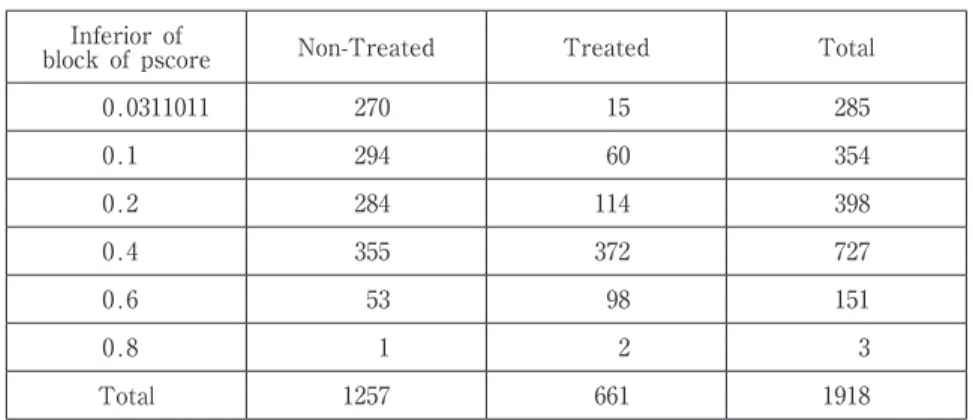
Before obtaining the ATT estimation, we predicted the propensity score by running the probit regression method. In this step, our estimation resulted in six blocks. This implies that the estimation of the propensity score s mean was not different in each block. Table 4 shows that the number of respondents in each group corresponds to their propensity score.
From the units available in each block, we estimated the ATT by subtracting their mean of outcomes. Moreover, we used the bootstrapping option up to 1,000 times to obtain the standard error (Table 4). From 1,257 individuals in the non-treated, we obtained 535 individuals as the control to 661 units in the treated. This estimation referred to the actual nearest neighbor matches.
With the standard error 0.18 and t-value −1.188 of estimation (Table 5), the negative result was not statistically significant at the 10 percent significance level. Therefore, we may not reject the null hypothesis that the program did not affect the education expenditure. More specifically, with PSM estimation, we may not conclude that on the average the beneficiaries had reduced their education expenditure if they participated in the program.
5―1―2 The Two-Stage Linear Squares Estimation
The empirical result of the 2SLS method in estimating the education expenditure is presented in Table 6. Before we had the results, we regressed the first stage using the probit method. By using the probit method in the first stage, we utilized four instrumental
Table 4. The inferior bound by Program Inferior of
block of pscore Non-Treated Treated Total
0.0311011 270 15 285 0.1 294 60 354 0.2 284 114 398 0.4 355 372 727 0.6 53 98 151 0.8 1 2 3 Total 1257 661 1918
Table 5. The ATT estimation with the Nearest Neighbor Matching method
Treated Control ATT Std. error t
661 535 −0.213 0.18 −1.188
variable derived from the participation of households in community activities. After testing the weak instrument, we provide the result of the first stage estimation in Appendix C. We tested the weak instrumental variable by using the likelihood ratio, Anderson-Rubin and Lagrange Multiplier method. Under the five percent significance level, except for the Anderson-Rubin, we rejected the null hypothesis that the beta value of the program variable was not different from zero.
The Tobit method was employed in the second stage because our dependent variable has the censored data observation, i. e., zero value. The main assumption of the Tobit method is that the decision to purchase and how much to purchase is solely based on the individual s preference. Furthermore, all coefficients explain the effect of an independent variable on the education expenditure per child.
However, we will not interpret the first stage estimation of this study because we just have to get the predicted value of this estimation in order to eliminate the endogenous
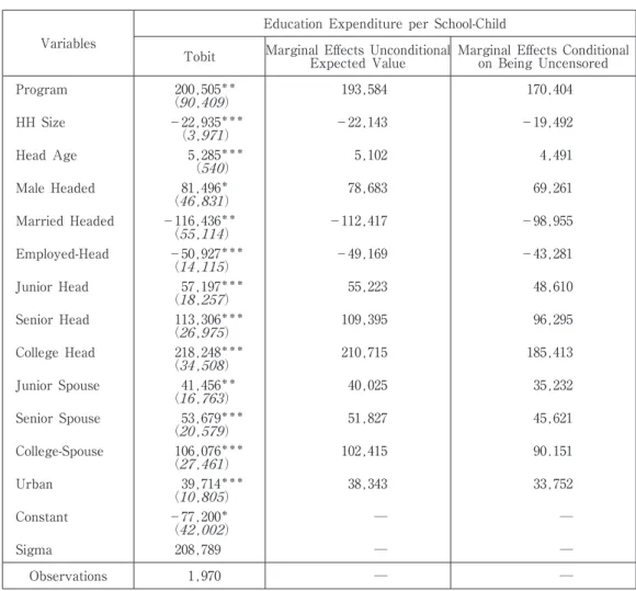
Table 6. Tobit Estimation and Marginal Effects of Education Expenditure Variables
Education Expenditure per School-Child
Tobit Marginal Effects UnconditionalExpected Value Marginal Effects Conditionalon Being Uncensored
Program 200,505*** ( , ) 193,584 170,404 HH Size −22,935*** ( , ) −22,143 −19,492 Head Age 5,285*** ( ) 5,102 4,491 Male Headed 81,496*** ( , ) 78,683 69,261 Married Headed −116,436*** ( , ) −112,417 −98,955 Employed-Head −50,927*** ( , ) −49,169 −43,281 Junior Head 57,197*** ( , ) 55,223 48,610 Senior Head 113,306*** ( , ) 109,395 96,295 College Head 218,248*** ( , ) 210,715 185,413 Junior Spouse 41,456*** ( , ) 40,025 35,232 Senior Spouse 53,679*** ( , ) 51,827 45,621 College-Spouse 106,076*** ( , ) 102,415 90.151 Urban 39,714*** ( , ) 38,343 33,752 Constant −77,200*** ( , ) ― ― Sigma 208,789 ― ― Observations 1,970 ― ―
Significance level at 0.10, 0.05, and 0.01 for*, ** and*** respectively
Numbers in parentheses are robust standard error Marginal effects was estimated by using dtobit2 in Stata.11
problem of the program in the outcome estimation. We use the predicted value of the first stage as replacing the program in the second estimation.
In order to explain the estimation of Tobit method, we need to examine the marginal effects of each variable. Table 6 provides the maximum likelihood estimation with the marginal effects of an unconditional expected value and the marginal effects of dependent on being uncensored, i. e., except zero value. All the marginal effects are conditional on education expenditure per child and calculated by the means of the independent variable. The interpretation of each variable is that an increase of the independent variable will affect the dependent variable for some amount, holding other variables constant at their means. Moreover, the marginal effect of the unconditional expected value is the average expenditure for all observations while the marginal effect of the conditional of being uncensored is for the observation above zero. Now, we will explain all variables based on the marginal effects in order.
The first column shows that under the 5% significant level the program shows a highly significant effect on the education expenditure. The second column implies that on average all participants have higher expenditure on education, about 193,584 rupiah, compared to non-participants. In addition, the uncensored participants increased their education expenditure about 170,404 rupiah if they participated in the program.
In general, the household and socio demographic variables show significant results. The household s size is statistically significant as expected. The negative sign means that the education expenditure decreases as the family size increases. The marginal effects of unconditional expected value explain that any additional member in the household will decrease the education expenditure of all respondents on average about 22,143 rupiah. In addition, with respect to the increasing family size, the uncensored respondent decreases its education expenditure about 19,492 rupiah.
The age of the head of the household has the opposite sign of the family size. This variable is highly significant as expected at 1% level. The result of the household s gender variable shows a positive significance at 10% level. On average, all respondents increase their education expenditure about 78,683 rupiah if the head of the household is male, The significant negative coefficient of married-headed household is contrary to our expected results. We were a bit surprised to find that the sign of working-headed household was similar to the married-headed household. This result is contrary to our expected result, as in general lower income relates to unemployment status.
The education level of the household s head and spouse show that this variable is so important to education expenditure. All levels of education are positive sign and are increasing. This was similar to the education level of the spouse.
The last variable shows that households that live in urban areas have more expenditure on education compared to the households that live in rural areas. This may be due to the fact that education facilities are better in urban areas than in rural areas (Tansel, 1998, and Kim and Lee, 2001).
5―2 Estimation of the Health Expenditure
In the health expenditure estimation, we used the same methodology of analysis as the education expenditure. We employed the PSM method to estimate the effect of
program in the health expenditure. With the same control variables from the household and demographic characteristics, we could not meet satisfactory matching levels, as the education expenditure did.
5―2―1 The Two-Stage Least Squares Estimation
Like in the previous outcome, we are also concerned with the endogenous program in the estimation. Table 7 presents the marginal effects at the observed censoring rate. We will interpret the marginal effects on the unconditional expected value and on the conditional of being uncensored. The first marginal effect refers to the average value of how the variable affects the outcome. This average value is from all respondents, including
Table 7. Tobit Estimation and Marginal Effects for the Health Expenditure Variables
Health Expenditure
Tobit Marginal Effects UnconditionalExpected Value Marginal Effects Conditionalon Being Uncensored
Program −20,568 (36,367) −18,040 −13,925 HH Size 7,458*** (1,620) 6,541 5,049 Head Age 1,009*** (162) 885 683 Male Headed −33,249*** (8,347) −29,163 −22,511 Married Headed 28,431*** (8,517) 24,938 19,249 Employed-Head 14,123*** (5,719) 12,387 9,562 Junior Head 10,860 (8,067) 9,525 7,352 Senior Head 16,809 (10,438) 14,743 11,380 College Head 28,581*** (12,838) 25,069 19,351 Junior Spouse 7,839 (8,012) 6,876 5,307 Senior Spouse 17,313*** (7,879) 15,186 11,722 College-Spouse 44,030*** (10,814) 38,620 29,811 Urban 12,729*** (5,462) 11,164 8,618 Constant −63,104*** (15,294) ― ― Sigma 169,932 ― ― Observations 6,429 ― ―
Significant at 0.10, 0.05, and 0.01 for*, ** and*** respectively
Numbers in parentheses are standard error
censored data. On the other hand, the latter marginal effect refers to the effects of variables which belong to uncensored units in the dependent variable. Now, we will explain all the independent variables in order.
The first column of the table shows that the program has a negative sign, but is statistically insignificant. We may say that the program does not appear to be associated with the increase of health expenditure. In other word, with the negative sign estimation we may not conclude that the program reduces the health expenditure of participant. Moreover, the unclear result is probably due to the condition that health expenditure is unpredictable. Therefore, the health expenditure is less likely to be a regular cost.
Unlike the education expenditure, the family size has a positive effect on health expenditure as expected. This variable implies that health expenditure increases along with the additional family member. The unconditional expected value is about 6,541 rupiah, which means that on average the respondents increase their health expenditure for additional members of the household. On the other hand, the uncensored respondents spend 5,049 rupiah on health as the size of the household increases. The effect of the head of the household s age is positively significant at 1% level. This implies that as the head of the household s age increases, the health expenditure increases as well. This finding is similar to Meng and Yeo (2005) who argued that in developing countries with undeveloped health systems, the older the head of the household, the higher the expenditure on health. Female-headed households seem likely to spend more on health expenditure than the male-headed households. The negatively significant coefficient of dummy male-headed at 1 % implies that the female-headed households pay more for the quality of their children than the male-headed households. This result is as expected and similar to other studies. The interpretation for unconditional marginal effects is, on average, the male-headed respondents spend less on health expenditure by about 29,163 rupiah than the female-headed households. On the other hand, the uncensored female-female-headed households are more likely to spend more on health expenditure by about 22,511 rupiah than male-headed households.
Marital status seems important to the health expenditure of households. The estimated coefficient is positively significant at 5% level as expected. It implies that married-headed households are more likely to spend more on the health expenditure than single-headed households. This result is the opposite of the education outcome.
Furthermore, the head of the household having a job significantly contributes to the health expenditure. This is true because the main variable affecting health expenditure is income. To interpret the result, the heads of household who are working on average spend more on the health expenditure by about 12,387 compared to the heads of household who are not working. On the other side, the uncensored heads of household who are working spend more on health expenditure, about 9,562 compared to the uncensored heads of household who are not working.
The college levels of the households heads shows a significant effect, which indicates that there is no evidence that less educated heads of household affect health expenditure.
In other words, the college level of the heads of household is the only variable that affects health expenditure. It is not similar to the spouses level of education. This variable is positively significant if the spouses are in the senior level of education and above.
In general, an urban residence does affect health expenditure compared to its counterpart. This result is similar to our expectation. A possible reason for this is that more health service choices with modern facilities are available in urban areas. In addition, households that live in rural areas are farther from the nearest health service. Moreover, according to a BPS survey in 2007, the main obstacle of households living in rural areas to access health services was income level, as well as availability of transportation and health service.
6
.Conclusion and Policy Implication
6―1 Conclusion
This study intends to analyze whether the Raskin program affected the expenditure of the participants, especially on education and health. Using the IFLS household data from the Rand Corporation, i. e., IFLS4 (2007), and employing the non-parametric and the semi-parametric approaches, this paper examines the contribution of the program to the expenditures of education and health.
Even though the data before 2007 are available (1993, 1997, and 2000), we only utilize the data in 2007 because we cannot capture the dynamics of the household such as death, newborn, newly married or separated, and many more. Therefore, we used the PSM method with the assumption that there is no baseline data. On the other hand, we employed the 2SLS method at the same time because we were concerned with the endogenous problem of the program.
The estimation results explain that the program does affect the participants expenditure on education, but not their health expenditure. This means that if the respondent participates in the program, he may increase his expenditure on education. This finding supports our hypothesis that the program contributed to education expenditure. However, we may not say that the program has impacted health expenditure because the estimated result is insignificant. One possible reason is that health expenditure is more likely a non-regular or unpredictable expenditure (David, 1993).
Relatively, all the households and demographic characteristics have significant and expected results except for the working head in the education outcome. These variable results are negative and statistically significant. A possible explanation is that the households head who were not working exploited their saving or wealth since they considered education to be important and they did not want their children to have a similar hardship in the future. However, we need further observation to discover the reason for our results.
members of households, and living in rural area, demonstrate the general characteristics of poor households. These factors relatively affect the participation in the program and the expenditure on education and health. Most importantly, the fact that higher-educated parents have spent more on education and health expenditure demonstrates that parents focus more attention on the quality of their children.
6―2 Suggestion and Policy Implication
The government of Indonesia has implemented the program with some characteristics for more than ten years. First, some ineligible households were exposed to the program, while some eligible households did not participate in the program, even though in general the participants were from the middle-income households. Regarding this condition, the government and NGOs should pay close attention to the process of targeting the beneficiaries. In addition, the poverty line used was still below 1.5 USD per capita per day, indicating that the method of targeting the beneficiaries did not describe the actual conditions of the poor households. Therefore, the method of 2,100 kilocalories consumption plus the non-food consumption should be improved by adding more food and non-food items as part of the estimation. All in all, the basic consumption per capita is close to the reality.
Second, the function of the program is not only for food security but also for redistribution income. The study revealed that its function as income has affected the education expenditure of the participants, even though the amount of the subsidy was still below the daily consumption. This contribution is not to health expenditure, because the health expenditure is more likely non-regular or unpredictable expenditure.
Parents consider education to be important for their children. Considering this, the government should support the fact that parents spend more of their expenditures on education. If it is possible, the government should provide education that is free of charge, with scholarships and other similar programs for the children of needy households.
Most of the participant heads of household worked. On the other hand, the study shows that non-working headed households spent more on education than those who were working-headed households. The possible explanation is that parents exploited their wealth for their children s education. Unfortunately, this behavior may cause other problems. Therefore, the government should implement other programs that generate income and create employment opportunities (Thwala, 2006).
Furthermore, providing programs empowering the spouse is also an alternative for poor households. Nowadays, empowering women through microcredit becomes popular in many developing countries. It is obvious that the low-level income households do not have access to credit. Therefore, providing loans to poor households is one solution to generate income. Many studies have proved that microcredit for the poor generated significant effects on the economy of poor households (Latifee, 2003 ; ADB, 2007).
The BPS data shows that the households expenditures on health are increasing. Meanwhile, our study reveals that the older the head of the household. the more the
expenditure on health. Therefore, the government should think of a way for poor people to get qualified health care without exploiting their wealth. Meng and Yeo (2005) suggested that in rural China with an undeveloped insurance system, elderly people tend to spend more on health. This indicates that providing health insurance for needy households at an early age should be a compulsory. If young people can access qualified health care, the possibility of better health outcomes is increased (Trujillo, Portillo, and Vernon, 2005 ; Martin, Rice, and Smith, 2007). Thus, elderly people can avoid depleting their wealth when they are old.
All of the programs suggested above rely on government spending. Other sectors that need improvement will lack of spending if the government allocates most of the budget for these kinds of programs. Therefore, accelerating economic growth could be another solution to alleviate poverty.
Moreover, human quality development will increase the skills of the people in the future, since most households already consider education and health to be important for their children. Education may increase the skills of workers, while health may increase the productivity of workers. These outcomes become incentive to attract more invesment. Furthermore, the higher the investment, the more likely the unemployment rate will decrease. On the other hand, the higher the skills and productivity of employers, the higher the income they can earn. This implies that people that are more educated and healthier can earn a higher income, which will raise their economic status.
6―3 Future Discussion
Program impact evaluation for the poor can yield a better result if we have the baseline data set. If we only use cross-section data, we cannot analyze the dynamics of the households. In other words, it is impossible to distinguish households who are living in the poverty status before and after the program, and which households were able to move out of poverty after the program.
Moreover, we employed the PSM method, which does not give clear-cut results. This could be because of the bias caused by self-selection bias or hidden bias in this study. Another possible explanation is that the study uses the comparison group from the same data source. In addition to that, we can also consider including more variables, with some possibility of variable interaction, and using other methods to get comparative results.
Acknon-ledements
This paper is a summary of the Master Thèsis written by Herbert Agust Suranta Munthe. The authors are grateful to Professor Kei Sakata for his constructive comments and insightful suggestions.
Notes:
* The views expressed on this paper are those of the authors and do not neccesarily represent those of the Indonesian Ministry of Finance Policy.
1) 1 USD=Rp. 9,000.00.
2) These contents are derived from the Bureau Central Statistic of Indonesia : 3) One can see the complete data at
4) The Governor of DKI Jakarta Regulation No. 93/2007 on Operational Guidelines on Rice for Poor Family Program (RASKIN) in 2007.
5) These contents are derived from the Ministry of Finance letter No : 117/PMK. 02/2007 on BULOG Budget Related to Stock and Distribution Management and Rice Price Stabilization. 6) These contents are derived from the Law No. 2/1989 and Law No. 20/2003 on National
Education System in Indonesia.
7) These contents are derived from the Socio and Demographic Health Census 2003, BPS. 8) All this information is derived heavily from IFLS4 : pp. 1―18. 9) The sample size below the poverty line that received the program was 77 households out of
661 households in the education outcome and 141 households out of 1,591 households in the health outcome.
10) We also applied the outliers exclusion based on 95 percent confidence level after estimating the predicted value.
11) The deeper explanation can be seen in Wooldrige (2002) : ―
12) The deeper explanation about the Tobit method can be seen in Cameron and Trivedi.
(2005) : ―
13) We used Stata.11 to utilize the raw data in all regression estimations. REFERENCES
Attanasio, O., and Mesnard, A. (2006). The impact of a conditional cash transfer program on consumption in Colombia. 27(4), 421―442.
Bryson, A., Dorsett, R., and Purdon, S. (2002). The use of propensity score matching in the evaluation of active labor market policies. Department for Work and Pensions.
Card, D. (1999). The causal effect of education on earnings. Orley Ashenfelter and David Card (eds.).
North-Holland, 3A, 1801―1863.
Chen, H. T. (1990). Newbury Park, CA : Sage.
Cochran, W. G., and Rubin, D. B. (1973). Controlling bias in observational studies : A review. 35A, 417―446.
Dehejia, R. H., and Wahba, S. (1999). Causal effects in non-experimental studies : Re-evaluating the
evaluation of training program. 94(448), 1053―
1062.
Dehejia, R. H., and Wahba, S. (2002). Propensity score matching methods for non-experimental
causal studies. 84, 151―161.
Diaz, J. J., and Handa, S. (2004). An assesment of propensity score matching as a non experimental impact estimator : Evidence from a Mexican poverty program. 41 (2), 319―345.
Donaldson, S. I. (2001). Mediator and moderator analysis in program development. In S. Sussman
Thousand Oaks, CA : Sage Publications, Inc.
Hastuti et al. (2007). The effectiveness of the program. SMERU Research Institute, Jakarta.
Hastuti, and Maxwell, J. (2003). Rice for poor family ( ) : Did the 2002 program operate effectively ? : Evidence from Bengkulu and Karawang. SMERU Research Institute, Jakarta.
Heckman, J. J., Hidehiko, H., and Todd, P. (1997). Matching as an econometric evaluation estimator : Evidence from evaluating a job training program. 64, 605―654. Heckman, J. J., Ichimura, H., and Todd, P. (1998a). Characterizing selection bias using experimental
data. 66(5), 1017―1098.
Heckman, J. J., Ichimura, H., and Todd, P. (1998b). Matching as an econometric evaluation estimator. 65, 261―294.
Hoddinott, J., and Skoufias, E. (2003). The impact of PROGRESA on food consumption. 53(1), 37―61.
Kim, S., and Lee, J. (2001). Demand for education and developmental state : Private tutoring in South Korea. The Paper is available at : http://papers.ssrn. com/paper.taf?abstract_id=268284
LaLonde, R. (1986). Evaluating the econometric evaluations of training programs with experimental
data. 76(4), 604―620.
Maluccio, J. A., and Flores, R. (2005). Impact evaluation of a conditional cash transfer program. The Nicaraguan Washington, DC, International Food Policy Research Institute (IFPRI).
Meng, X., and Yeo, C. (2005). Ageing and health-care expenditure in urban China. Departement of Economics, Reasearch School of Pacific and Asian Studies, Australian National University. Parker, Susan, W., and Wong, R. (1997). Household income and health expenditures inMexico.
40, 237―255.
Rosenbaum, P. (2002). (2nd ed.). New York : Springer.
Rosenbaum, P., and Rubin, D. (1983). The central role of the propensity score in observational studies for causal effects. 70(1), 41―55.
Rossi, P. H., Lipsey, M. W., and Freeman, H. E. (2004). ( ) Thousand Oaks, CA : Sage.
Rubin, D. B. (1974). Estimating causal effects of treatments in randomized and nonrandomized
studies. 66(5), 688―701.
Rubin, D. B. (1979). Using multivariate matched sampling and regression adjustment to control bias
in observational studies. 74, 318―328.
Rubin, D. B. (1997). Estimating causal effects from large data sets using propensity scores. 127, 757―763.
Sackey, H. A. (2007). The determinants of school attendance and attainment in Ghana : A gender perspective.
Sumarto, S., Suryahadi, A., and Widyanti, W. (2004). Assessing the impact of Indonesia social safety net program on household welfare and poverty dynamics.
17(1), 155―157.
Tansel, A. (1998). Determinants of school attainment of boys and girls in Turkey. 21, 455―470.
health. 29(4), 950―988.
Tilak, J. B. G. (2002). Determinants of household expenditure on education in rural India. National Council of Applied Economic Research.