トップページ - 横浜国立大学学術情報リポジトリ

(1)

Abstract

　　The nature of trade and production in East Asia has undergone many changes over the past few decades. While a lot of researchers have examined the nature of these changes, there have been only few attempts at reviewing the existing results to ascertain the present state of research. The objective of this paper is to fill this important gap by linking the methodologies and results of most cited research in this area. This review underlines the rising importance of vertical production networks and intermediate goods trade in Asia. The main methodology used in literature to quantify this vertical specialization of trade is through an analysis of international input-output tables. Such an analysis of vertical specialization through input-output tables for East Asia shows that even though China takes the position as the main supplier in East Asia, there is high degree of import content in Chinese export to the world. This paper also identifies the scope for future research. This review finds that given the development of new and improved methodologies for quantifying vertical specialization and value added trade, there is a need to relook at many conventional approaches and indices of macroeconomics using value added exports data rather than the commonly used gross exports data. Secondly, the impact of value added trade on the different components of value added like labor incomes or capital incomes can also be developed for future research. Lastly, we find much of the existing literature on production networks look at trade from the perspective of parent country. There is need for more theoretical explanation on the benefits of joining production network from the view point of a host country.

Keywords: East Asia, Fragmentation, Vertical Specialization, Value- Added Trade 1．Introduction: Terms and Concepts

　　The current trade pattern in East Asia is best explained by a rise in interconnected vertical network trade in intermediate goods extending across various countries of East Asia. It can be seen as a conveyor belt which passes through many countries, with each country adding value to the good at various upstream or downstream stages of production.1)_{Given this rising interconnected network of trade, various researchers have identiﬁed}

The Importance of Vertical Production Networks and

Intermediate Goods Trade in Asia: A Literature Review

Simi Thambi

1) This is different from the regional transmission pattern of Flying Geese (FG) theory originally developed by Akamatsu (Akamatsu, 1962) and it extension by Kojima (Kojima, 2001) to explain the trade patterns of the early decades of East Asian industrialization. The idea of third stage of FG theory of regional transmission involved:

(2)

62 Yokohama Journal of Social Sciences, Vol. 19, No. 3

that an understanding of the implications of this network trade on traditional idea of trade is the need of the hour. However to know implications, the first step is to understand thoroughly the idea of vertical production network trade. Therefore the aim of this paper is to review some of the most cited literature in the field of vertical production network trade. The objective is to give the reader a concise summary of the main debates and results of the literature in this field, as well as identify the various methodologies used to quantify this phenomenon.

　　There are some terms that are often used in the literature on this field. Figure 1 provides a schematic illustration of the distinction of these terms in the context of production networks. The figure has three columns: Trade, FDI and production networks in East Asia.

　　Trade is defined as export or import of goods. Foreign Direct Investment (FDI) is defined as investment in foreign countries through licensing or setting up affiliates. Figure 1 shows that the first set: International trade can be of two types – inter-industry trade or one way trade and intra-industry trade. Inter-industry trade refers to the trade of goods among different industries of different countries. For e.g. 　　　　　　　　　

　・Trade in ﬁnal goods 　・Inter-Industry trade

　・Country as the unit of Analysis

In contrast, the current trade patterns in East Asia are characterized by: 　・Trade in intermediate goods

　・Intra-Industry trade 　・Firm as the unit of analysis

For more on this debate, refer Uemura (2014). Furthermore, Uemura (2014) brings out a clear distinction between Akamatsuʼs original version of FG theory and its extension by Kojima. While Akamatsuʼs version saw trade in the Ricardian model of trade. Kojimaʼs extension saw FG theory in a Hecksher-Ohlin framework with factor price differences and factor price equalization. Uemura (2014) argues that the original Akamatsuʼs FG theory with wage differentials is more appropriate to explain the current pattern of production networks trade in Asia.

1 Simi Thambi 図表

Figure 1 Schematic Illustration of Keywords Based on a Literature Review

Source: Author

Figure 2 The Fragmentation Theory: Production Blocs and Service Links

Source: Jones and Keirzkowski (1990). as depicted in from Ando and Kimura (2011)

One Way

Trade/

Inter industry

Trade

Intra industry

Trade(IIT)

Horizontal IIT

Verical II

T

Vertical FDI

FDI

Horizontal FDI

Vertical FDI

Production

Networks

in

East Asia

Vertical IIT

（214）　Source: Author

(3)

63 The Importance of Vertical Production Networks and Intermediate Goods Trade in Asia（Simi Thambi）

if there are two countries: country 1 and country 2; trade of goods from the agriculture industry of country 1 for goods from the machinery industry of country 2. Another kind of trade is intra industry trade. For e.g. goods from country 1ʼs machinery industry are traded for goods from country 2ʼs machinery industry. Intra industry trade can further be divided into horizontal and vertical trade. Horizontal trade is the case where goods are differentiated by attributes. Vertical trade is the case where goods are differentiated by quality.

　　The second set in Figure 1 shows FDI. Some firms may find it profitable to undertake foreign direct investment in other countries. They can do this either by licensing to the firms in the host country or by setting up the affiliates of the parent firm in the host country.2)_{In both cases the nature of FDI can be either horizontal} or vertical. Horizontal FDI refers to the case when firms enter the host country with a market seeking objective. Vertical FDI refers to the case when the firms enter the host country with the objective of saving costs.3) 　　A review of literature on production networks in East Asia shows that the definition of production networks in Asia does not fit completely into just one of these sets .i.e. only trade or only FDI. The nature of production network in East Asia includes components of both these sets. Production network trade in Asia can be seen mainly as the subset of vertical intra industry trade and vertical foreign direct investment.4)_{Intra-Industry trade} because much of the East Asian network trade deals with the parts and components of the machinery sector. 　　The rest of this paper is organized as follows. Section 2 presents a review on the growth of production network trade and vertically specialized intermediate goods trade. Section 3 reviews the methodology of research used in literature to quantify vertical specialization. Section 4 looks at the role of Japan and China in these vertical production networks. Section 5 concludes all the above sections and identifies scope for future research.

2．Growth of Vertical Production Network Trade and Vertically Specialized Intermediate Goods Trade 　　Origins of international production networks have been traced to activities of MNCs from US. However, until the 1980s the nature of this trade was mainly a north-north trade between North America and European Nations. Overtime these ﬁrms began to explore opportunities in North South trade in the neighboring countries of Latin and South America. Unfavorable investment climate in those countries induced these MNCs to look towards East Asia and South East Asia (UNESCAP; 2011). Consequently there was a rapid increase in production networks in East Asia by middle of 1990s facilitated by the favorable investment and trade policies of these countries. A lot of researches have been done to investigate these new patterns of trade in East Asia. This section attempts to link the ﬁndings of some most cited research in explaining current trend of increased 　　　　　　　　　

2) For details refer Ownership, Location, Internalization Theory (OLI Theory) (Dunning, 2001).

3) Some authors argue it is difﬁcult to clearly distinguish between these two types of FDI as sometimes both these kinds of FDI coexist. For e.g. Japanese automobile assemblers are taking advantages of regional trade liberalization programs to set up production facilities in ASEAN countries and facilitate the division of labor within the region, in order to achieve a regional scale of production (UNESCAP, 2011). Nevertheless, we believe the initial motive of entry is Vertical FDI even though at some point of time later the MNC may engage in horizontal FDI. Furthermore most literature on IPN (International Production Network) see vertical FDI as an important feature of IPN and not horizontal FDI.

4) Vertical FDI eventually expands to include horizontal FDI in some cases.

(4)

fragmentation and vertical production.5)

2. 1 Reason for the Existence of Production Networks: Fragmentation Theory

　　The reason for the existence of production network trade is best explained by the theory of fragmentation of a ﬁrm. The pioneer attempt to explain this theory was made by Jones and Keirzkowski (1990). His idea is presented through a schematic illustration as shown in Figure 2.

　　Figure 2 shows the case of a firm before and after fragmentation. The upper part shows the case before fragmentation. This figure consists of a big rectangle which is divided into smaller rectangles and squares. Assuming the big rectangles represents a firm that produces a single product. The smaller squares and rectangles are production blocs (PB). “Production blocs represent the different kinds of tasks that go into producing that product”. Each bloc can have different characteristics; it can be purely capital intensive, labor intensive or a mix of both. Under some circumstances, it is economical for the firm to separate these production blocs and locate them elsewhere in different host countries.

　　The lower part of the figure shows the case of a firm after fragmentation. “Each production block is now separated and linked to each other through arrows which are called service links (SL)”. Firms will choose to fragment their production process into production blocs if it is technically feasible and economically profitable. Technical feasibility refers to the technical separability of the production bloc from the main production process. Economic profitability means the separation of production blocks is more profitable than when in a single integrated production process framework. This happens because of two reasons. Either when there is a high efficiency of production costs due to the location advantages of the host country to which the production bloc is

1 Simi Thambi 図表

Figure 1 Schematic Illustration of Keywords Based on a Literature Review

Source: Author

Figure 2 The Fragmentation Theory: Production Blocs and Service Links

Source: Jones and Keirzkowski (1990). as depicted in from Ando and Kimura (2011)

One Way

Trade/

Inter industry

Trade

Intra industry

Trade(IIT)

Horizontal IIT

Verical II

T

Vertical FDI

FDI

Horizontal FDI

Vertical FDI

Production

Networks

in

East Asia

Vertical IIT

　Source: Jones and Keirzkowski (1990). as depicted in Ando and Kimura (2011)

Figure 2 The Fragmentation Theory: Production Blocs and Service Links

5) Ando and Kimura (2011) make a similar attempt at reviewing literature. However it is felt that their reviews fails to include some important researches. Even though some debates may appear the same, the value addition of this paper over the aforementioned paper is that it tries to include most cited important researches in this ﬁeld.

(5)

moved or when the service link costs incurred in connecting remotely located production blocs are small. These service link costs depend not only on trade barrier and transport cost but also on various coordination costs. 2. 2 Ways of Fragmenting Production in Production Network Trade: Vertical Intra-Industry Trade

and/or Vertical FDI

　　In the context of production networks, there are two main ways in which the firm can fragment its production blocs. The literature on this ﬁeld points towards two main activities in this respect, vertical intra industry trade and vertical FDI. Figure 3 explains this idea using the example of 2 countries, parent country and host country.6)_{Parent country can fragment its production to the host country in two ways via arms length} transactions with host country firms or by setting up multinational affiliates of the parent firm in the host country. The choice of internalization is primarily the parent ﬁrmʼs choice.7)

　　Figure 2 and Figure 3 taken together explain in a simple framework, the interactions between 2 countries. In reality however the idea is much more complicated with many countries and hence intricate networks of ﬁrms.

2.3 Result of Fragmentation: Growth of Trade in Intermediate Goods Trade or Vertically Specialized Intermediate Goods Trade?

　　Fragmentation involves the breakup of the production process into fragments of tasks that produce 　　　　　　　　　

6) Ando and Kimura (2011) in Figure 4 provide an illustration of two dimensional fragmentation. 7) For details on this refer literature on the theory of internalization of OLI paradigm (Dunning, 2001).

　Source: Author

Figure 3 Fragmentation between the Parent and Host Country in East Asia: Vertical Intra Industry Trade and Vertical FDI

（217）

2 Figure 4 Flowchart of Literature on Production Networks and Growth of Trade

Source: Author

Table 1 VS Exports as a Share of Merchandise Exports

Source: Chen et al. (2005) Pg 42 VS exports as a share of merchandise exports

HOST COUNTRY PARENT COUNTRY Parent Firm Export/ Import Vertical Intra Industry Trade

Vertical FDI into the host

country

Production Networks

Intermediate Goods

Vertically Specialized goods

Multinational Enterprise (MNE) of Parent Firm (Cross border intra ﬁrm fragmentation) Host Country Firm (Cross border arm’s length fragmentation)

(6)

different kinds of intermediate goods8)_{which joined together result in the production of the final good. Many} intermediate goods can go into the making of a final good. Moreover, each intermediate good can further be used in the production of other intermediate goods. This creates an interconnected network of production extending across different countries. Vertically specialized intermediate goods can be defined as a subset of intermediate goods, those goods which cross multiple countries for different stages of production.9)

　　Trade in intermediate goods has increased significantly in the past two decades. Some critics argue that a large part of the growth in world trade in the past decades can be attributed to the growth in the trade of intermediate goods. Trade flows are dominated not by goods that are fully consumed but by goods that are further used in the production of other goods and services. Intermediate inputs represent 56% of total goods trade and 73% of total services trade in 2009. The trade of intermediate inputs has grown at an average annual rate of 6.2% for goods and 7% for services (in volume terms) between 1995 and 2006. However, trade in final goods and services has increased at the same pace and as a consequence, the share of intermediate goods trade in total trade has remained constant while the share of intermediate services trade has slightly increased (Miroudot et al. 2009). Other studies also confirm the growing importance of intermediate goods trade (Ng and Yeats 2001, 2003; Athukorala and Yamashita, 2006).

　　However, some critics argue that main reason for growth of world trade in the past decades is the increase in the trade of a subset of intermediate goods that they call vertically specialized intermediate goods. They argue that the share of intermediate goods in total trade has remained constant. In fact it is the share of vertically specialized intermediate goods those intermediate goods that cross multiple borders that has been increasing.

　　Figure 4 shows the flow chart of the scope of literature on production networks in the order of their importance in production network trade. The literature on production networks ﬂows from intermediate goods to vertical specialized intermediate goods. In other words, within the trade in production networks, the most important category that has led to growth of trade is intermediate goods and even within that it is vertically specialized goods that are most prominent.

　　Yi (2003) in his famous magniﬁcation effect analysis asserts that it is vertically specialized goods which cross multiple borders that explain most of the growth of world trade. Magniﬁcation effect is the magnifying effect of tariff reductions into large increases in trade when goods cross the borders of multiple countries. For instance, if there are N sequential stages each in a different country, a one percent decrease in tariff will

（218）

8)An intermediate good is defined as an input to the production process that has itself been produced and, unlike capital, is used up in production. The difference between intermediate and capital goods lies in the latter entering as a fixed asset in the production process. Like any primary factor (such as labor, land, or natural resources), capital is used but not used up in the production process. On the contrary, an intermediate good is used, often transformed, and incorporated in the final output. As an input, an intermediate good has itself been produced and is hence defined in contrast to a primary input. As an output, an intermediate good is used to produce other goods (or services) contrary to a final good which is consumed and can be referred to as “consumption good”). For e.g. the production of a car require tires which requires steel and rubber; steel requires iron which requires iron ore and so and on, similarly rubber requires other inputs. This is a definition provided by Deardorff (2006) in his Glossary of International Economics.

9) A good is called vertically specialized when three conditions are met: (1) a good (or service) is produced in two or more sequential stages; (2) two or more countries provide value-added during the production process; and (3) at least one country uses imported inputs in the process and some of the output is exported” (OECD and WTO, 2012).

(7)

cause the cost of production to reduce by N% (in contrast to a 1% decline in the cost of a regular traded good). This is the reason why the degree of increase in world trade over the past few decades is much more than can be explained by decrease in tariffs, in other words the extent of increase in world trade is much larger than can be explained by the tariff reduction in standard trade models. He shows this by including the idea of vertical specialization in a 2 country dynamic Ricardian trade model with three stages of production: primary, intermediate and ﬁnal goods.

　　Bridgman (2012) agrees with the above and extends his study to argue that magnification effect is most significant in manufactured intermediate goods. In his study he presents a three stage vertical specialization Ricardian trade model of raw materials, manufactured parts and ﬁnal goods sectors by looking at the exchanges between the home and foreign country with two households in a tractable general equilibrium framework for world trade during the period 1967 to 2002. Through his simulated trade model he looks at growth in world trade and changes in the composition of trade. At the sector level, manufacturing trade tripled while overall trade growth only doubled. Within the manufacturing sector, in the category of intermediate goods, his results show that raw materials share of intermediate goods trade have decreased while the share of manufactured goods in intermediate goods has increased. Within the share of manufactured goods in intermediate goods, the share of vertically specialized goods is rising rapidly. Even though at the overall level, the share of intermediate goods in total trade has been constant. He avers that lower trade costs on manufactured parts led to Vertical Specialization (VS) trade growth.

　　Chen et al. (2005) also ﬁnds that trade of intermediate goods to total trade has not increased but a subset of trade in intermediate goods which deals with the trade of vertically specialized goods has increased. Table 1 shows vertically specialized (VS) exports as a share of merchandise exports has increased for 10 OECD countries for the period 1968 to 1998.

　　According to another prominent study by Yeats (2001), vertically specialized intermediate goods trade is most prominent in the parts and component industry. Yeats (2001) in his pioneer study looks at the commodity composition of global production sharing. His results pointed towards the importance of trade in components within the entire machinery and transport (SITC 7) sector.

　　To sum up, in this section, we saw that the reason for production network trade is best explained by the

2 Figure 3 Fragmentation between the Parent and Host Country in East Asia: Vertical Intra Industry

Trade and Vertical FDI

Source: Author

Figure 4 Flowchart of Literature on Production Networks and Growth of Trade

Source: Author

Table 1 VS Exports as a Share of Merchandise Exports

Source: Chen et al. (2005) Pg 42 VS exports as a share of merchandise exports

HOST COUNTRY MNE of Parent Firm ( Cross border intra firm fragmentation)

Host Country Firm

(Cross border arm’s

length ragmentation)

PARENT COUNTRY Parent Firm Export/ Import Vertical Intra Industry Trade

Vertical FDI into the host

country

Production Networks

Intermediate Goods

Vertically Specialized goods

Figure 4 Flowchart of Literature on Production Networks and Growth of Trade

　Source: Author

(8)

fragmentation theory of production that splits production blocs across national borders. The ﬁrms mainly use vertical FDI and vertical intra-industry trade to fragment production. Finally, we highlighted the growing importance of vertical specialization in intermediate goods of parts and components facilitated by reduction in tariffs and transport costs. In the next section, we will review the main methodology used in literature to quantify this phenomenon of vertical specialization.

3．Methodology to Quantify Vertical Specialization

　　With the rising importance of vertical specialization in international trade many researchers have identified ways to quantify this phenomenon. The main methodology used is through an analysis of international input-output tables. Table 2 lists the main databases used by researchers in this ﬁeld.

　　The development of literature on quantifying vertical specialization originated from the pioneer work of Hummels et al. (2001). In the years that followed, this method was extended by several researches like Johnson and Noguera et al. (2012, 2014), Koopman et al. (2012, 2014) and Strehrer (2012, 2013). The objective of this section is to review the main results and link the methodologies used by all the above mentioned authors.

（220）

Table 1 VS Exports as a Share of Merchandise Exports

(9)

3. 1 Foundation Measure of Vertical Specialization

　　Hummels et al. (2001) made one of the ﬁrst attempts to quantify vertical specialization. There are two ways in which a country can be engaged in vertical specialization:

　　・By using imported intermediates to produce exports

　　・ By exporting intermediate goods which are used as inputs by other countries to produce goods for export.

　　He represented the former as VS and the later as VS1. However he developed a clear mathematical formula only for the former leaving the latter for future research.10)

　　His model was formulated as a two country case for vertical specialization. Such a model can be used to look at the interaction of two countries with each other or one country interaction with the world aggregated as the other country. For two countries r and s and one sector, vertical specialization (VS) in terms of import content of export of country r can be formulated as:

VSr =

VS r= �imported intermediates_{gross output} sr

r � .exportsrs = VSn Xn= ∑ VSn rn ∑ Xn rn = μAM X Xn rn μAM _X Xn μAM ( I-AD)-1X Xr

And ∑ VSn r= ∑ �n imported intermediates_{gross output} sn� .exports_rn=μAM X

VAX= va12

x12=

r1�s� y12�s�

x12�s� (2)

�A_A11 A12

21 A22� is the input coefficient matrix

V(I-A)-1Y E or

VBY E

　　This equation shows the ratio of imported intermediates in the total output of country r multiplied by the exports from country r to s.

　　For a case of n sectors, aggregate Vertical Specialization (VS) for country r is the sum of imported intermediates from country s to r across all sectors n divided by total exports of all sectors for country r,

Aggregate VSr =

VS r= imported intermediates_{gross output} sr

r .exportsrs = VSn_X n= ∑ VSn r ∑ Xn r = μAM X Xn rn μAM X Xn μAM _{( I}_－_AD₎－1_X Xn

And ∑ VSr= ∑ imported intermediatessi

i gross output . n n exportsis=μAM X VAX= va12 x12= r1s y12s x12s (2) A11 A12

A21 A22 is the input coefficient matrix

V(I－A)－1Y E or

VBY E

Where,

Xn is a scalar representing the sum of country r exports

Table 2 Different Input-Output Datasets

Name of Dataset Key Features

Global Trade Analysis Project Database Input-output tables for over 100 countries for various benchmark years, mostly after 2000. https://www.gtap.agecon.purdue.edu

World Input-Output Database Global tables covering OECD countries and major emerging markets from 1995–2011. http://www.wiod.org

IDE–JETRO Asian Input-Output Tables Regional tables covering 8 East Asian countries at ﬁve-year intervals between 1985 and 2000.

http://www.ide.go.jp

OECD Input-Output Tables Input-output tables for OECD countries and major emerging markets, available various years from

1970–2005.

http://www.oecd.org /trade/input-outputtables.htm 　Source: Adapted from Johnson (2014) Table 1, Pg. 123

10) VS1 was clearly formulated by his successor Koopman et al. (2010, 2012, 2014).

(10)

70 Yokohama Journal of Social Sciences, Vol. 19, No. 3 And

r .exportsrs = VSn Xn= ∑ VSn r ∑ Xn r = μAM _X Xn rn μAM X Xn μAM _{( I}_－_AD₎－1_X Xn

V(I－A)－1Y E or VBY E Where, μ is a 1×n unit vector

AM_{is the n×n import coefﬁcient matrix}

X is an n ×1 vector of exports, n is the number of sectors i is a representative sector of country r

　　In the above equation

r � .exportsrs = VSn_X n = ∑ VSn rn ∑ Xn rn = μAM X Xn rn μAM X Xn μAM _{( I-A}D₎-1_X Xr

And ∑ VSn r= ∑ �n imported intermediates_{gross output} sn� .exportsrn=μAM X

VAX= va12

x12=

r1�s� y12�s�

x12�s� (2)

�A11 A12

A21 A22� is the input coefficient matrix

V(I-A)-1Y E or

VBY E

captures the direct import content of exports (expressed as the share of intermediate imports over total exports) but it does not reflect how imported intermediates are used indirectly throughout the economy. To capture the indirect use of imported intermediates at different stages of domestic production, before these are embodied in an export flow, Hummels introduced the Leontief inverse matrix [I－ AD_]－1_{to the above expression. Here A}D_{is an n x n domestic technical coefficient matrix which reflects the value of} domestic intermediates over total output (rather than imported intermediates over imported intermediates which was used in the case in the AM_{matrix). Adding this Leontief inverse to the above equation captures the use of} imported intermediates across each stage of domestic production allowing the imported input to be embodied in a domestic output at the 2nd_{, 3}rd_{, 4}th_{, . . . stage before it becomes embodied in the good that it is exported.}

　　Therefore ﬁnally the, HYI VS Index (Hummels et al. (2001) Vertical Specialization Index) can be written as:

　　　　　　　HYI VS Share of Total Exports =

r .exportsrs = VSn Xn= ∑ VSn r ∑ Xn r = μAM X Xn rn μAM X Xn μAM ( I－AD)－1X Xn

V(I－A)－1Y E or

VBY E

(1)　 Where, u is a 1×n unit vector, AM_{is the n×n imported coefﬁcient matrix, I is the identity matrix, A}D_{is the} n × n domestic coefficient matrix, X is an n×1 export vector, Xn is the total country exports and n is the

number of sectors.

　　The above mentioned HYI VS index made the hallmark attempt at quantifying the import content of export or VS, a sequence of vertical specialization which was hitherto unmeasured. However it had some limitations which are as follows:

　　・ HYI VS captures the import content of export assuming only one country exports intermediate goods. Therefore whenever both the countryʼs export intermediate goods, the model diverges from the real import content of export.

　　・ It uses the assumption that imports are 100% foreign sourced, in other words it does not take into account that some inputs might be reﬂected back after processing abroad.

　　・ HYI VS measure is an aggregate measure it shows the intermediate imports from all countries into home country embodied in the exports to all countries however it does not measure the bilateral degree of vertical specialization.

　　The researches that followed, improved upon the limitations in the following ways:

　　・ To overcome the first limitation, the definition of exports was broadened to include the export of intermediate goods by both countries.

　　・ The second limitation arose because in the case of HYI VS, only the import coefﬁcient matrix was used （222）

(11)

to calculate the direct import content of export, assuming all imported content was foreign value added with no domestic value added and all the foreign value originated in one country. However this is not the case in the real world. We can show this with an example.

　　　Consider the following three cases:

　　　 Case 1: Direct Import: For instance, US imports from China a good that is completely made in China, 100% Chinese value added.

　　　 Case 2: Import includes goods reﬂected back to home country: For instance, US imports from China a good that has Chinese value added and US value added that returns back to US after being processed in China. 　　　 Case 3: Import includes reﬂected back imports plus indirect imports: In the Case 2 above, if Chinese

value added consists of parts imported from other Asian countries, then that means US is indirectly importing the value added of those countries.

　　　 To measure the above mentioned sequences of trade, researches identiﬁed that it is best to use the direct domestic value added vector. This is one of the main differences between older literature on vertical specialization and newer literature on value added to measure vertical specialization.

　　・ To overcome the third limitation, i.e. to change the HYI measure from aggregate to bilateral, two methods have been used in literature. One way is by using the proportionality assumption. The proportionality assumption assumes that the intensity in the use of intermediate inputs is the same between production for exports and production for domestic sales. The other way is to use detailed end use classification (intermediate or final) of detailed import statistics like BEC (Business Economic Classification). The second method is increasingly used by researches rather than the conventional proportionality assumption. 3.2 Value added Trade and Vertical Specialization

　　Given the limitation of the VS measure mentioned in the previous section, the researches that followed identiﬁed that the best way to look at vertical specialization was to look at it through value added in trade, i.e. by making use of the value added coefﬁcient vector provided in any input-output table.11)

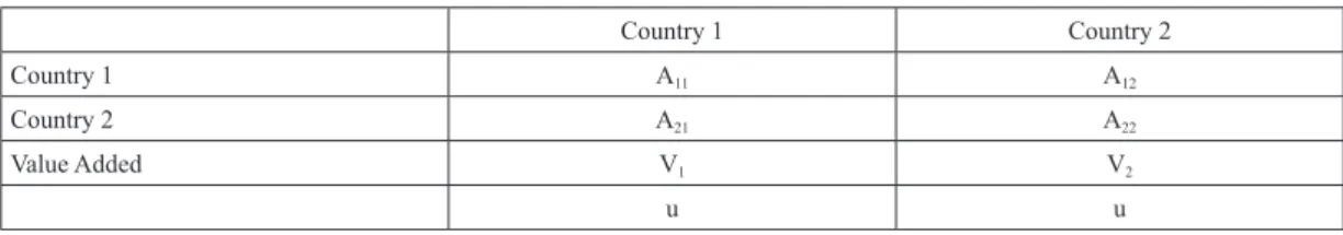
　　Table 3 attempts at linking direct value added vector and import coefﬁcient vector used by HYI VS using a two country simple Input-Output Model:

　　In a country with just 2 sectors, u is a 1×2 row vector, u=(1,1)

Table 3 Simple Two Country 1 Unit Output I-O Representation

Country 1 Country 2 Country 1 A11 A12 Country 2 A21 A22 Value Added V1 V2 u u 　Source: Author 　　　　　　　　　

11) A detailed examination of all the proofs of the mentioned in the literature on this ﬁeld is beyond the scope of this paper. This paper will only look at the main measurement equations of different methodologies.

(12)

r � .exportsrs = VSn Xn= ∑ VSn rn ∑ Xn rn = μAM _X Xn rn μAM _X Xn μAM _{( I-A}D₎-1_X Xr

VAX= va12

x12=

r1�s� y12�s�

x12�s� (2)

�A_A11 A12

V(I-A)-1Y E or

VBY E

is the input coefﬁcient matrix

　　The economic explanation of this is that, to produce one unit of output in country 1, country 1 requires units of domestic goods and units of imported intermediate goods. Therefore the fraction of domestic output that represents domestic value added in country 1 is V1= u－uA11－uA21. Similarly we can arrive at direct value added vector for country 2.

　　It is easy to see from the above equation the connection between domestic and import coefﬁcient matrix and direct value added coefﬁcient vector. In the remaining part of this section, we will review the prominent literature that uses this direct value added vector to quantify domestic and foreign value added.

　　・ Johnson (2012) is famous for his measure called VAX ratio (Value added to exports ratio). VAX ratio is deﬁned as the ratio of direct domestic value added to gross exports. For a two country case (1,2) with sectors (s, s ) respectively using the terminology used in his paper, VAX can be written as:12)

r � .exportsrs = VSn_Xn =∑ VSn rn ∑ Xn rn = μAM _X Xn rn μAM X Xn μAM _{( I-A}D₎-1_X Xr

VAX= va12

x12=

r1�s� y12�s�

x12�s� (2)

�A_A11 A12

V(I-A)-1Y E or

VBY E

⑵　　　r1 [s] is payment to domestic factors or domestic value added. It is the direct value added row vector. (Its general form can be expressed as ri [s]=1－∑j ∑s Aji [s, s]. In this equation ri [s] is payment to domestic factors. ∑s stands for summation of imports from all sectors of country j ∑j stands for summation of imports from all countries j to country i.)

　　y12[s] is called implicit output transfer from country 1 to country 2. The output from country 1 directly and indirectly used to produce ﬁnal goods absorbed in country 2. It can be written as y12[s]= (I－A)－1Y12, where Y12 is direct export by country 1 in the form of ﬁnal demand of country 2 and (I－A)－1_{is the Leontief inverse which} shows the intermediate inputs that were indirectly used in making Y12.

　　X12[s] is the gross bilateral export from country 1 to country 2 including export of intermediate goods and export of ﬁnal goods.

　　・ Koopman et al. (2010, 2012, and 2014) is one of the latest methodologies in the literature on vertical specialization and value added. It currently forms the base of all calculations related to recent value added in databases like OECD TIVA and UNCTA GVC database. In their ﬁrst paper Koopman et al. (2012) extended on the work of Hummels et al. (2001) and Johnson (2012) to decompose value added into different sequences, for the ﬁrst time in literature.

　　The literature that uses this methodology has two related branches. VAiT (Value added in Trade) and TIVA (Trade in Value Added). Before we proceed, it is important to have a clear idea of the differences between these two concepts which look very similar. Table 4 presents a concise summary of the main differences between the two approaches.

　　 For this paper, we are mainly interested in the source of value added from the viewpoint of vertical production networks. Therefore we focus on reviewing the Koopman (2010, 2012 and 2014) methods to quantify VAiT or Value Added in Trade.

（224）

12) Based on the explanation of this equation, it is easy to see that VAX ratio=

r .exportsrs = VSn Xn= ∑ VSn r ∑ Xn r= μAM X Xn rn μAM X Xn μAM _{( I}_－_AD₎－1_X Xn

And ∑ VSr= ∑ imported intermediatessi i gross output . n n exportsis=μAM X VAX= va12 x12= r1s y12s x12s (2) A11 A12

V(I－A)－1Y E or

VBY E (using

(13)

　　Koopman et al. (2010) contributed to the existing literature by decomposing the gross exports of a country into value added components by source.

　　Assuming all gross output produced by country r must be used as an intermediate good or ﬁnal good at home or abroad. For a two country case, gross output equation for country r can be written as follows:

11 ൬X_X1₂൰ = ൬A_A11 A12 21 A22൰ ൬ X₁ X2൰ + ൬ Y₁₁+Y₁₂ Y21+Y22൰ ൬X1 X2൰ = ቈ I-A₁₁ -A₁₂ -A₂₁ I-A₂₂቉ -1 ൬Y11+Y12 Y21+Y22൰ = ൬ B₁₁ B₁₂ B21 B22൰ ൬ Y₁ Y2൰ VAS=VB= ൬V1B11 V1B12 V2B21 V2B22൰ Where V= ൬V₀1 _V0

2൰ is the direct value added coefficient diagonal matrix

VAiT = VBE = ൬V1B11 V1B12 V2B21 V2B22൰ ൬ E₁ 0 0 E2൰ = ൬ V₁B₁₁E₁ V₁B₁₂E₂ V2B21E1 V2B22E2൰ (3) VB= ቌ V₁B₁₁ V₁B₁₂ V₁B₁₃ V₂B₂₁ V₂B₂₂ V₂B₂₃ V3B31 V3B31 V3B33 ቍ (3a) E = ൭EE1*1* EE2*2* EE3*3* E_1* E_2* E_3*൱ (3b) VBE = ቌVV1₂BB₂₁11EE_1*1* VV1₂BB12₂₂EE_2*2* VV₂1BB₂₃13EE3*_3* V₃B₃₁E_1* V₃B₃₁E_2* V₃B₃₃E_3*ቍ (3c) X_r=A_rrX_r+ A_rsX_s+Y_rr+Y_rs　　　　(r, s=1,2) (r, s=1,2)

Where Xr is N×1 gross output vector of country r, Arr is the N×N domestic input coefficient vector, Ars isN× N input coefficient matrix giving intermediate use in country s of goods produced in country r, Yrr is the N×1 domestic final demand vector, Yrs isN×1 final demand vector in country s for final goods from country r. The two country production and trade system can be written in block matrix form as follows:

11 X1 X₂ = AA1121 AA1222 X1 X₂ + YY11₂₁+Y+Y12₂₂ X1 X₂ = I－A₁₁ －A₁₂ －A21I－A₂₂ －1 Y11+Y12 Y₂₁+Y₂₂ = BB11₂₁ BB12₂₂ YY1₂ VAS=VB= V1B11 V1B12 V₂B₂₁ V₂B₂₂ Where V= V1 0

0 V₂ is the direct value added coefficient diagonal matrix

VAiT = VBE = V1B11 V1B12 V₂B₂₁ V₂B₂₂ E0 E1 0₂ = VV1₂BB11₂₁EE₁1 VV1₂BB12₂₂EE2₂ (3) VB= VV12BB1121 VV21BB2212 VV21BB1323 V₃B₃₁ V₃B₃₁ V₃B₃₃ (3a) E = EE1*1* EE2*2* EE3*3* E1* E2* E3* (3b) VBE = V1B₁₁E1* V1B₁₂E2* V1B₁₃E3* V2B21E1* V2B22E2* V2B23E3* V3B31E1* V3B31E2* V3B33E3* (3c) Xr=ArrXr+ ArsXs+Yrr+Yrs (r, s=1,2)

Table 4 Differences between VaiT and TIVA

VaiT (Value added in Trade) TIVA (Trade in Value Added). Deﬁnition Value Added in Trade (VaiT) measures

the domestic and foreign value added content of trade.

Trade in Value added (TIVA) measures how much of value added of a particular country is contained in the consumption of another country.

The emphasis here is on the source of

value added The emphasis here is on the destination of where value added by a particular country is consumed

Formula VBE

where,

V= Value Added Coefﬁcient Matrix B= Leontief Inverse Matrix

E= AX+ F( AX is intermediate good export and F is ﬁnal good exports)

VBY where,

V= Value Added Coefﬁcient Matrix B= Leontief Inverse Matrix Y= Final Demand Treatment of Intermediate Exports and

Final good Export Includes intermediates in ExportsE= AX+ F Excludes intermediates,Includes only Final Demand. Diagonal Elements Diagonal elements show domestic Value

Added Content of Exports Diagonal elements show Value Added absorbed at Home Off diagonal Elements Off diagonal elements show foreign

Value Added Content of Exports Off diagonal elements show export of Domestic Value Added to other countries

Column Sum Gross Exports Final Demand

Compiled Databases UNCTAD-EORA GVC Database

For 187 countries from 1990-2010 WTO-OECD TIVA DatabaseFor 57 countries in 1995, 2000, 2005, 2008 and 2009.

http://stats.oecd.org 　Source: Author

(14)

74 Yokohama Journal of Social Sciences, Vol. 19, No. 3 　　This system can also be succinctly expressed as follows:

X = (I – A)－1_{Y = BY, Where B stands for Leontief Inverse Matrix (I – A)}－1 Using this share to create VAS (Value added share) matrix deﬁned as:

VAS=VB= 11 ൬X_X1 2൰ = ൬ A11 A12 A21 A22൰ ൬ X1 X₂൰ + ൬YY11₂₁+Y+Y12₂₂൰ ൬X_X1 2൰ = ቈ I-A₁₁ -A₁₂ -A21 I-A22቉ -1 ൬Y_Y11+Y12 21+Y22൰ = ൬ B11 B12 B₂₁ B₂₂൰ ൬YY1₂൰ VAS=VB= ൬V1B11 V1B12 V2B21 V2B22൰ Where V= ൬V1 0

0 V₂൰ is the direct value added coefficient diagonal matrix

VAiT = VBE = ൬V1B11 V1B12 V₂B₂₁ V₂B₂₂൰ ൬E0 E1 0₂൰ = ൬VV1₂BB11₂₁EE₁1 VV1₂BB12₂₂EE2₂൰ (3) VB= ቌ V1B11 V1B12 V1B13 V2B21 V2B22 V2B23 V₃B₃₁ V₃B₃₁ V₃B₃₃ቍ (3a) E = ൭EE1*1* EE2*2* EE3*3* E1* E2* E3* ൱ (3b) VBE = ቌ V1B11E1* V1B12E2* V1B13E3* V2B21E1* V2B22E2* V2B23E3* V3B31E1* V3B31E2* V3B33E3* ቍ (3c) Xr=ArrXr+ ArsXs+Yrr+Yrs (r, s=1,2) Where V= 11 ൬X_X1 2൰ = ൬ A11 A12 A21 A22൰ ൬ X1 X2൰ + ൬ Y11+Y12 Y21+Y22൰ ൬X_X1 2൰ = ቈ I-A₁₁ -A₁₂ -A₂₁ I-A₂₂቉ -1 ൬Y_Y11+Y12 21+Y22൰ = ൬ B11 B12 B21 B22൰ ൬ Y1 Y2൰ VAS=VB= ൬V1B11 V1B12 V₂B₂₁ V₂B₂₂൰ Where V= ൬V1 0

0 V2൰ is the direct value added coefficient diagonal matrix

VAiT = VBE = ൬V1B11 V1B12 V2B21 V2B22൰ ൬ E1 0 0 E2൰ = ൬ V1B11E1 V1B12E2 V2B21E1 V2B22E2൰ (3) VB= ቌ V₁B₁₁ V₁B₁₂ V₁B₁₃ V2B21 V2B22 V2B23 V3B31 V3B31 V3B33 ቍ (3a) E = ൭EE1*_1* EE2*_2* EE3*_3* E_1* E_2* E_3*൱ (3b) VBE = ቌ V₁B₁₁E_1* V₁B₁₂E_2* V₁B₁₃E_3* V₂B₂₁E_1* V₂B₂₂E_2* V₂B₂₃E_3* V3B31E1* V3B31E2* V3B33E3* ቍ (3c) X_r=A_rrX_r+ A_rsX_s+Y_rr+Y_rs (r, s=1,2)

is the direct value added coefﬁcient diagonal matrix

　　Based on this VB foundation, Koopman et al. (2012) developed two measures: VAiT & TIVA. In this paper, we focus on Value Added in Trade.

　　　　　　　　　VAiT = VBE = 11 ൬X1 X2൰ = ൬ A₁₁ A₁₂ A21 A22൰ ൬ X₁ X2൰ + ൬ Y₁₁+Y₁₂ Y21+Y22൰ ൬X_X1 2൰ = ቈ I-A₁₁ -A₁₂ -A₂₁ I-A₂₂቉ -1 ൬Y_Y11+Y12 21+Y22൰ = ൬ B11 B12 B21 B22൰ ൬ Y1 Y2൰ VAS=VB= ൬V1B11 V1B12 V2B21 V2B22൰ Where V= ൬V₀1 _V0

2൰ is the direct value added coefficient diagonal matrix

VAiT = VBE = ൬V1B11 V1B12 V2B21 V2B22൰ ൬ E1 0 0 E2൰ = ൬ V1B11E1 V1B12E2 V2B21E1 V2B22E2൰ (3) VB= ቌ V₁B₁₁ V₁B₁₂ V₁B₁₃ V2B21 V2B22 V2B23 V3B31 V3B31 V3B33 ቍ (3a) E = ൭EE1*_1* EE2*_2* EE3*_3* E_1* E_2* E_3*൱ (3b) VBE = ቌ V₁B₁₁E_1* V₁B₁₂E_2* V₁B₁₃E_3* V₂B₂₁E_1* V₂B₂₂E_2* V₂B₂₃E_3* V3B31E1* V3B31E2* V3B33E3* ቍ (3c) X_r=A_rrX_r+ A_rsX_s+Y_rr+Y_rs (r, s=1,2) (3)　 Where Ers =∑s (Ars Xs+Yrs), in other words, export of intermediate goods and ﬁnal goods from country r to country s

　　From equation (3), we can see two sequences, the diagonal terms V1 B11 E1, V2 B22 E2 are domestic value added and off-diagonal terms V2 B21 E1, V1 B12 E2 are foreign value added for country 1 and country 2 respectively.

　　Similarly, in the case of three countries we can write equation (3) as follows, 　　　　　　　VB= 11 ൬X_X1 2൰ = ൬ A11 A12 A21 A22൰ ൬ X1 X2൰ + ൬ Y11+Y12 Y21+Y22൰ ൬X_X1 2൰ = ቈ I-A₁₁ -A₁₂ -A₂₁ I-A₂₂቉ -1 ൬Y_Y11+Y12 21+Y22൰ = ൬ B11 B12 B21 B22൰ ൬ Y1 Y2൰ VAS=VB= ൬V1B11 V1B12 V2B21 V2B22൰ Where V= ൬V1 0

VAiT = VBE = ൬V1B11 V1B12 V2B21 V2B22൰ ൬ E1 0 0 E2൰ = ൬ V1B11E1 V1B12E2 V2B21E1 V2B22E2൰ (3) VB= ቌ V₁B₁₁ V₁B₁₂ V₁B₁₃ V2B21 V2B22 V2B23 V3B31 V3B31 V3B33 ቍ (3a) E = ൭EE1*_1* EE2*_2* EE3*_3* E_1* E_2* E_3*൱ (3b) VBE = ቌ V₁B₁₁E_1* V₁B₁₂E_2* V₁B₁₃E_3* V₂B₂₁E_1* V₂B₂₂E_2* V₂B₂₃E_3* V3B31E1* V3B31E2* V3B33E3* ቍ (3c) X_r=A_rrX_r+ A_rsX_s+Y_rr+Y_rs (r, s=1,2) (3a)　　　　　　　E = 11 ൬X_X1 2൰ = ൬ A11 A12 A21 A22൰ ൬ X1 X2൰ + ൬ Y11+Y12 Y21+Y22൰ ൬X_X1 2൰ = ቈ I-A₁₁ -A₁₂ -A21 I-A₂₂቉ -1 ൬Y_Y11+Y12 21+Y22൰ = ൬ B11 B12 B₂₁ B₂₂൰ ൬YY1₂൰ VAS=VB= ൬V1B11 V1B12 V₂B₂₁ V₂B₂₂൰ Where V= ൬V1 0

VAiT = VBE = ൬V1B11 V1B12 V2B21 V2B22൰ ൬ E1 0 0 E2൰ = ൬ V1B11E1 V1B12E2 V2B21E1 V2B22E2൰ (3) VB= ቌ V1B₁₁ V1B₁₂ V1B₁₃ V2B21 V2B22 V2B23 V3B31 V3B31 V3B33 ቍ (3a) E = ൭EE1*_1* EE2*_2* EE3*_3* E1* E2* E3* ൱ (3b) VBE = ቌ V₁B₁₁E_1* V₁B₁₂E_2* V₁B₁₃E_3* V2B21E1* V2B22E2* V2B23E3* V3B31E1* V3B31E2* V3B33E3* ቍ (3c) Xr=ArrXr+ ArsXs+Yrr+Yrs (r, s=1,2) (3b)　　　　　　　VBE = 11 ൬X_X1 2൰ = ൬ A11 A12 A21 A22൰ ൬ X1 X2൰ + ൬ Y11+Y12 Y21+Y22൰ ൬X_X1 2൰ = ቈ I-A₁₁ -A₁₂ -A21 I-A₂₂቉ -1 ൬Y_Y11+Y12 21+Y22൰ = ൬ B11 B12 B₂₁ B₂₂൰ ൬YY1₂൰ VAS=VB= ൬V1B11 V1B12 V₂B₂₁ V₂B₂₂൰ Where V= ൬V1 0

VAiT = VBE = ൬V1B11 V1B12 V₂B₂₁ V₂B₂₂൰ ൬E0 E1 02൰ = ൬ V1B11E1 V1B12E2 V₂B₂₁E₁ V₂B₂₂E₂൰ (3) VB= ቌ V1B11 V1B12 V1B13 V2B21 V2B22 V2B23 V3B31 V3B31 V3B33 ቍ (3a) E = ൭EE1*_1* EE2*_2* EE3*_3* E1* E2* E3* ൱ (3b) VBE = ቌ V₁B₁₁E_1* V₁B₁₂E_2* V₁B₁₃E_3* V2B21E1* V2B22E2* V2B23E3* V3B31E1* V3B31E2* V3B33E3* ቍ (3c) Xr=ArrXr+ ArsXs+Yrr+Yrs (r, s=1,2) (3c)　 Where E1* is the sum of country 1ʼs exports to country 2 and country 3. E2* is the sum of country 2ʼs exports to country 1 and country 3. E3* is the sum of country 3ʼs exports to country 1 and country 2.

　　From equation (3c), we can see three sequences, domestic value added in exports, foreign value added in exports and indirect value added exports.

　　The diagonal terms measure domestic value added exports (DV).

DVr = Vr Brr Er* FVr = ∑ Vs≠r sBsrEr* IVr = ∑ Vs≠t rBrsEst E_r*=DV_r+ FV_r Er*=Vr Brr∑ Ys≠r rs + Vr Brr∑ As≠r rs Xss +Vr Brr∑ As≠r rs Xst +Vr Brr∑ As≠r rs Xsr +FV E1_{= �} E₁₂+E₁₃ -E₂₁ -E₃₁ �

　　The sum of off-diagonal elements along a column is the true measure of value added from foreign sources (FV) embodied in a particular countryʼs gross exports.

(15)

DV_r = V_r B_rr E_r* FV_r= ∑ Vs≠r sBsrEr* IVr = ∑ Vs≠t rBrsEst Er*=DVr+ FVr Er*=Vr Brr∑ Ys≠r rs + Vr Brr∑ As≠r rs Xss +Vr Brr∑ As≠r rs Xst +Vr Brr∑ As≠r rs Xsr +FV E1_{= �} E12+E13 -E₂₁ -E₃₁ �

　　The sum of off-diagonal elements along a row provides indirect value added (IV) which is a countryʼs value added embodied as intermediate inputs in third countries̓ gross exports or indirect value added exports.

DVr = Vr Brr Er* FVr = ∑ Vs≠r sBsrEr* IV_r = ∑ Vs≠t rBrsEst E_r*=DV_r+ FV_r E_r*=V_r B_rr∑ Ys≠r rs + Vr Brr∑ As≠r rs Xss +Vr Brr∑ As≠r rs Xst +Vr Brr∑ As≠r rs Xsr +FV E1_{= �} E12+E13 -E₂₁ -E₃₁ �

　　The sum of a column is the sum of domestic value added and foreign value added, which is nothing but the total exports of a particular country. Its general form can be expressed as

DV_r = V_r B_rr E_r* FV_r= ∑ Vs≠r sBsrEr* IVr = ∑ Vs≠t rBrsEst Er*=DVr+ FVr Er*=Vr Brr∑ Ys≠r rs + Vr Brr∑ As≠r rs Xss +Vr Brr∑ As≠r rs Xst +Vr Brr∑ As≠r rs Xsr +FV E1_{= �} E12+E13 -E₂₁ -E₃₁ �

　　The above equation can further be decomposed into the following form: 　　　　　　　 DVr = Vr Brr Er* FVr = ∑ Vs≠r sBsrEr* IV_r = ∑ Vs≠t rBrsEst E_r*=DV_r+ FV_r Er*=Vr Brr∑ Ys≠r rs + Vr Brr∑ As≠r rs Xss +Vr Brr∑ As≠r rs Xst +Vr Brr∑ As≠r rs Xsr +FV E1₌ E₁₂+E₁₃ －E₂₁ －E₃₁ (4) 　　The ﬁrst four terms are the components of which can be understood as follows: 13)

1．Vr Brr ∑s≠rYrs = Exported in ﬁnal goods (Direct value added export)

2．Vr Brr ∑s≠rArs Xss = Exported in intermediates absorbed by direct importers (Direct value added export) 3．Vr Brr ∑s≠r Ars Xst= Exported in intermediates re-exported to third countries (Indirect value added exports) 4．Vr Brr ∑s≠r Ars Xsr= Exported in intermediates that return back

Where

Summing up 1, 2, 3 divided by gross exports gives the VAX ratio which is formalized by Johnson and Noguera (2012) , as seen in equation (2)

Summing 3 and 4 gives HYI VS1 which is mentioned in Hummels et al. (2001) Furthermore, in the equation (4) is HYI VS measure

　　Koopman et al. (2012, 2014) extended on the analysis of Koopman et al. (2010) in mainly two ways. First, they clearly identiﬁed which parts of ofﬁcial trade data are double counted and what is the source of this double counting.Second, they further decomposed foreign value added into its components. Figure 5 presents an idea of the extensions of Koopman et al. (2014) over Koopman et al. (2010).14)

　　・ Stehrer (2012, 2013) calculated VAiT in a different way from the Koopman et al. (2010, 2012, and 2014) method. Their measure emphasizes on the net value added in trade. The main differences are summarized as follows:

　　　 Firstly, the export matrix is different in Stehrer (2012, 2013) compared to Koopman et al. (2010, 2014). This can be clearly seen by looking at the export matrix for a three country case. The vector of gross trade for country 1 can be written as,

（227）

13) For details on calculation see Koopman et al. (2012) Pg. 14. A detailed exposition of all the formulas is beyond the scope of this paper.

(16)

76 （228） Yokohama Journal of Social Sciences, Vol. 19, No. 3

5 Figure 5 Koopman et al. Methodology

1. Koopman et al. (2010)

2. Koopman et al. (2014)

5 Figure 5 Koopman et al. Methodology

1. Koopman et al. (2010)

2. Koopman et al. (2014)

Figure 5 Koopman et al. Methodology

1. Koopman et al. (2010)

(17)

E1₌ DV_r = V_r B_rr E_r* FV_r= ∑ Vs≠r sBsrEr* IVr = ∑ Vs≠t rBrsEst Er*=DVr+ FVr Er*=Vr Brr∑ Ys≠r rs + Vr Brr∑ As≠r rs Xss +Vr Brr∑ As≠r rs Xst +Vr Brr∑ As≠r rs Xsr +FV E1₌ E12+E13 －E₂₁ －E₃₁

Where, E includes both intermediate exports and ﬁnal good exports denoted as E=AX+Y. Using the same logic for the other two countries, three country matrix E* _{can be written as follows:}

　　　　　　　Export matrix E*₌ 15 Export matrix E*₌ E12+E13 －E12 －E13 －E₂₁ E₂₁+ E₂₃ －E₂₃ －E₃₁ －E32 E31+E32 (4)

tVaiT, Netr =V I－A －1 E*_{= i}─ _{I－A I－A}－1_E*_{= i}─ _E*_{= t} Gross, Net r 1+IVir Eir －Ln( 1+ FVir Eir) (5)　

　　Note the difference between this new E*_{matrix and in the case of Koopman (2010, 2014) in equation (3b). Post} multiplying this new E*_{matrix with VBS matrix in the equation (3a), we get the Strehrer version of VB E}*_matrix. 　　The second difference between the two methodologies is that the sum of the each column of E*_{matrix in} the case of Stehrer (2012, 2013) is equal to the net trade balance. This can be easily seen from equation (5). And the sum of each column of VBE*_{is equal to the net value added trade balance. On the other hand, the sum} of the column elements of Koopman et al. (2010, 2014) VBE matrix in equation (3c) is gross exports.

　　Thirdly, in Stehrer (2012, 2013) the sum of column elements of export matrix is equal to column elements of value added matrix. In other words, the net trade balance is equal to the value added trade balance for all countries.15)

Discussion on Stehrer (2012, 2013) and Koopman et al. (2010, 2012, and 2014):

　　Kuboniwa (2014), using Strehrer (2012, 2013), produced an interesting result that showed the bilateral equivalence between TIVA and VAiT in net value added trade. He argued that this condition of bilateral equivalence cannot be proved using the Koopman et al. (2010, 2012, and 2014) method. He thus avers that for the calculation of net value added trade, Strehrer (2012, 2013) has an advantage over Koopman et al. (2010, 2012, and 2014) method. 　　Kuboniwa (2014) result is unique in its ﬁnding; nevertheless we wish to highlight the importance of the original Koopman et al. (2010, 2012, and 2014) methodology over previous methodologies. Koopman et al. (2010, 2012, and 2014) method has a number of advantages over Strehrer (2012, 2013). It has the ability to quantify measures like: domestic value added, foreign value added, indirect value added, exports reflected back and also double counted term. Furthermore, for the ﬁrst time in the literature of international trade, the above mentioned components of gross exports could be decomposed at both bilateral and multilateral level. Appendix 1 presents a numerical example to compare Koopman et al. (2010, 2012, and 2014) with Strehrer (2012, 2013) method. According to OECD and WTO (2011), Koopman et al. provides a full decomposition of value-added exports in a single conceptual framework that encompasses all the previous measures. However this report points to areas in which the Koopman et al. methodology can further be extended. They mention that Koopman et al. method does not account for different kinds of domestic value added, “domestic value-　　　　　　　　　

15) This can be seen by the expression, using the deﬁnition of value added.

15 Export matrix E*₌ E12+E13 －E12 －E13 －E₂₁ E21+ E23 －E₂₃ －E₃₁ －E32 E31+E32 (4)

tVaiT, Netr =V I－A－1E*= i─ I－A I－A－1E*= i─ E*= tGross, Netr

1+IVir

Eir －Ln( 1+

FVir

Eir )

Here i denotes a 1 × n summation vector. V is the direct value added coefﬁcient diagonal matrix. E* is equation (5). （229）

(18)

added” can be found indirectly in imports of foreign inputs (as ʻreturned domestic VAʼ) and when exported to another country can be also indirectly found in exports from third-countries.16)_{Furthermore, they bring to} notice that the next step in the analysis is to provide a full decomposition of the foreign value-added according to the country of origin of the VA. This follows from equation (3b). For instance, exports of country 1 are expressed as which is the sum of exports of country 1 to country 2 and country 3.

　　To conclude in this section, we discussed mainly four methodologies that have been used in literature to quantify vertical specialization and value added trade. Hummels et al. (2001) made the pioneer attempt at quantifying vertical specialization but his index included restrictive assumptions which resulted in double counting and were not applicable in the real world. His research was extended by researches like Johnson (2012), Koopman et al. (2010, 2012, and 2014) and Stehrer (2012, 2013). Out of all these, the most elaborate methodology seems to be that of Koopman et al. (2010, 2012, and 2014). This is because for the ﬁrst time in literature it was able to quantify measures like: domestic value added, foreign value added, indirect value added, exports reﬂected back and also double counted term.

4．Role of Japan and China in Vertical Production Networks and Intermediate Goods Trade 　　Both Japan and China have an indispensable role in East Asian production networks. This section reviews the results of literature using the methodology mentioned in the previous section. Our objective for this section is to identify the role of Japan and China in the vertical production networks.

　　Dean et al. (2008) quantiﬁed the import content of Chinese processing exports and normal exports using Hummel et al. (2001) methodology for the period 1997 and 2002, by sector and trading partners using detailed Chinese Input Output Database for 1997 and 2002. Their main result was that Chinaʼs trade is becoming more vertically specialized, between 1997 and 2002 Chinaʼs VS share increased by about 23%. The most vertically specialized sectors in Chinaʼs trade are plastics, steel processing, communications equipment, industrial machinery, metal products, and electronic computers. In these sectors, imported intermediate goods account for between 52 percent and 76 percent of the value of Chinese exports. Within that the wholly-owned foreign ﬁrms and joint ventures have the most vertically specialized trade. There is a strong evidence of Asian network of suppliers to China, Japan and the Four Tigers account for more than half of the value of Chinaʼs imported inputs both in 1997 and in 2002. They identify Hong Kong, the US, and Singapore as being the most vertically specialized among Chinaʼs export destinations.

　　Baldwin and Gonzalez (2013) develop the Hummel et al. (2001) to decompose the sourcing patterns of intermediate imports used by China for US exports. Figure 6 presents their result. The height of each bar shows the share of Chinaʼs exports to the US made up of imported intermediates. The bars also show where the imported intermediates are sourced from. Their ﬁnding is in tandem with Dean et al. (2008). Japan, Taipei and Korea stand out as main countries from which China imports intermediate inputs for export to US.17)

（230）

16) OECD and WTO (2012, Pg. 20).

17) This results is in synch with the theoretical argument of Yun (2000) in his study about Asian production patterns where he argued that what can be seen in East Asia is a system of hierarchical complex production links which are connected vertically backwards to Japan due to dependence on exports of Japanese technology and vertically forward to US due to its continuing position as the main external export market for East Asian manufacturers.

(19)

　　Johnson et al. (2014) look at the sector level export shares for China in gross and value added terms using VAX ration of Johnson et al. (2012). They ﬁnd that in the Electrical and Optical equipment industry, the real value added by China is less than half of the total gross exports in that industry. Furthermore they look at the share of Electrical and Optical Equipment in value-added and gross exports over time. The share of this sector in gross exports has almost doubled since 1995, while the value-added share has barely changed.

　　Koopman (2008, 2010, 2012 and 2014) using Dean et al. (2007) methodology of breaking down Chinaʼs total exports into processing exports and normal exports, found that domestic value added in Chinaʼs processing exports is much lower than that in Chinaʼs normal exports. For e.g. in 2004 domestic value added in Chinaʼs normal exports was 44.2% while for Chinaʼs processing exports the ﬁgure was only 28.8%.18)_{Furthermore, it is} interesting to see that the returned domestic value added is only 0.3% and 1.2 % for Chinaʼs normal exports and processing exports respectively. On the other hand for advanced countries like Japan, Western EU and US, this returned domestic value added share of gross exports is much greater at 2.9%, 7.4% and 12.4% respectively. In addition, Koopman et al. (2010) computed a country sector-level index for position in global value chain called GVC_positon. It is defined as log ratio of a country-sectorʼs supply of intermediates used in other countriesʼ exports to the use of imported intermediates in its own production. If the country lies upstream in a supply chain in other words, is the supplier of intermediate inputs, the numerator is large. On the other hand if it is downstream then the denominator is large.19)_{Their results showed that for electronic equipment sector, Japan is one of the} most upstream countries along with Western EU, US and Mexico. China on the other hand is one of the most

（231）

18) For detailed decomposition of gross exports of all countries for the year 2004, see Koopman (2008, 2010, 2012 and 2014). 19) GVC_positon= Ln 15 Export matrix E*₌ E12+E13 －E12 －E13 －E₂₁ E21+ E23 －E23 －E₃₁ －E32 E31+E32 (4)

tVaiT, Netr =V I－A－1E*= i─ I－A I－A－1E*= i─ E*= tGross, Netr

1+IVir Eir －Ln( 1+ FVir Eir) Koopman et al. (2010) Pg. 21.

6 Figure 6

Import Content in Chinese Exports to the US

Source: Baldwin and Gonzalez(2013) Figure 34. Using OECD IO table