Linking National Econometric Models of Japan, U. S. A., and the East and Southeast Asian Countries : A Pilot Study

Southeast Asian Studies, Vol. 17, No.2, September 1979

Linking National EconolD.etric Models of Japan,

U.S.A., and the East and Southeast Asian

Countries

-A Pilot Study-*

Mitsuo EZAKI

**

I Introduction

The East and Southeast Asian countries have close economic realtions with Japan and the United States through trade and capital movements. Quantitative anal-ysis and forecasting of any national economy, therefore, cannot be made properly without allowing for its inter-dependent relations with other economies. The Project LINK (Ball [1973], Wael-broeck

[1976],

etc.) is the world-wide research effort which focuses on this as-pect of economic interdependency mainly among developed countries in the world. Developing countries are considered only on the aggregate regional basis. For ex-ample, all of the South and East Asian countries are aggregated into a single region, for which only an aggregate regional model is constructed based on the average data of the region.I) Not

• This research was done as one of the pilot studies for the link project organized and headed by Professor Shinichi Ichimura, from whom the author received many useful com-ments and advices. The author, however, is solely responsible for any errors in the paper.

•• rr_J't!1J, The Center for Southeast Asian Studies, Kyoto University

1) See \Vaelbroeck [1976J, pp.397-409. In

to mention the heterogeneity of the individual countries, those who wish to analyze Asian economic problems can not be satisfied with the aggregate results for the region.

The Center for Southeast Asian Studies, Kyoto U niversi ty is now attempting to develop a system of linking national econometric models of East and Southeast Asian countries with those of their major trading partners, i.e., Japan and the United States. The present paper is an outcome of this research project. Since its purpose is to investigate the basic nature and merits of the linked system including Japan, U.S.A. and some East and Southeast Asian countries as a pilot study, it has several limitations in scope and analysis. First, the countries covered in this study are only four: Taiwan, Korea, the Philippines and Thailand. Second, a simple prototype modle, i.e.,

a ten-equations system of the effective demand type, is employed commonly as Project LINK, the developing countries are classified into four regions: (a) Latin America, (b) South and East Asia, (c) Middle East and Libya, and (d) Africa excluding Libya.

M. EZAKl: Linking National Econometric Models the country model not only £Ix the four

countries mentioned above but also for Japan and U.S.A.2) Third, exports and imports are treated only in total,

i.e.,

no disaggregation by SITe numbers, and the linkage is allowed only for trade relations, 'toe., no capital transactions introduced. Finally, the model here is used for the analysis of economIC interdependency based on policy simulations, but not for the forecasting purposes. These limi-tations in scope and analysis may look senous. However, the link-model de-veloped here can still be favorably com-pared with the unlinked country model in deriving some basic facts and policy implications which underlie the inter-dependent relations among Japan, U.S.A. and several East and Southeast Asian countries.3)

In Section 2, we will propose a pro-totype model for linkage and discuss about an iterative method to get the solution of the model. In Section 3, we will provide the ordinary least squares (OLS) estimates of structural equations and check the simulatability of the model from the point of view of the final test or dynamic simulations. In Section 4, on the basis of this dynamic simulations, we

2) The country model in the present paper is quite similar to the model proposed by Klein and Van Peeterssen [1973] tentatively for France and Italy, in which suitable models were not yet available at the time of starting Project LINK.

3) The present study owes much to the papers collected in Ball [1973] and Waelbroeck [1976]. Moriguchi [1973] and Gana, Hickman and Lau [1977] are also important sources of reference.

will quantify the effects of the changes In policy variables, t.e., government consumption expenditures and exchange rates, and analyze the repercussions among the countries. We will also com-pare the simulation results of the linked

Table 1 A Prototype Model for Linkage

Country Model (i=I, ... , N-l)*

(C-l) n=q+lt+Gf+X~-Mf (C-2) X~(PX~/r~)f)i=X$f+XS$f

(C-3) M~(PM~/r~)(Ji=M$f+MS$~ (C-4) C~=fCYf,Ci-1> 15lJMU (C-5) If=fCYL liUMn

(C-6) X$f=fCWT$t, X$f-l, PX$UPW$tJ (C-7) M$~=f[Y~(PYUr~)Oi,M$f-l'

PM$f(rfIr~)/(PYfIPY~)J (C-8) PYf=fC YU Yt, (PM$V PM$t)(iUrDJ (C-9) PXf=fCPYf, (PW$t!PW$b)(rUrDJ

(C-IO) PX$: =f[(PXUPX~)/ (rUr~)J

Trade .Model (Linkage)

(T-l) X$f l =fCY{(PYtlrt)(jJ, X$f~l,PX$UPM$f, PX$f(T{ /r;)/(PY{ /PY~)J (i,j = 1...N - 1; i"'-\cj) (T-2) X$fJ_{=A1${-L:.f",,-lX$f}J (j=1...N-l) (T-3) X$fN=X$i-L:.1:1X$fl (i=l. .. N-l) (T-4) X$fN=ac·WT$, (T-S) PX$fJ=PfJ·PW$c (j=1...N) (T-6) M$f=L:.f=lX$f N (T-7) X$f=L:/f=lX$f J (T-8) PX$f=L:.!J=lPX$fJ·X$fJ IL:.1=lX$!jJ (T-9) WT$t=L:f=lXSf(=L:!J=lM${) (T-10) PW$t= L:.f=lPX$f·X$UL:.f=lX$f (T-ll) Plv/${= (L:f=-lPX$f·X$fj +PX$f J .X$fl)/L:.f=lX$fl (j=l.ooN)

*

i= 1: Japan (jPN) , i=2: U.S.A. (USA),

i=3: Taiwan (TWN), i=4: Korea (KREA),

i= 5: Philippines (PHIL), i= 6: Thailand (THAI), and i=N=7: Rest of the World (ROW).

system with those of the unlinked country model. In Section 5, some concluding

remarks will be given.

II A Prototype Model for Linkage

Table summarIzes the prototype model for linkage which is employed in the present paper. The corresponding notation is shown in Table 2. Our model for linkage consists of two parts: country model and trade model. The country

model is a sys tern of ten equations (C-I)--(C-IO), for which the linear form will be assumed in estimation (i.e., f (A, B, ) means the linear function of A, B, ). The ten-equations system is commonly used for each of the sixc ountries under

Table 2 Notation of the Link Model*

Country i:

Y = GNP or GDP at constant prices (NIs)a C = Private consumption expenditures

at constant prices ( " )

I = Gross domestic capital formation at constant prices ( " )

G

= Government consumption expendi-tures at constant prices ( " )

X = Exports of goods and services at constant prices ( " )

M = Imports of goods and services at constant prices ( " )

PY = Implicit deflator of GNP or GDP (

"

PX = Implicit deflator of exports of goods and services ( " )

*PM = Implicit deflator of imports of goods and services ( " ) r = Exchange rate per US$

(UN Statistical Yearbook) 8 = Scale factor which adjusts NIS data to trade data (Table 4)

DUM = Dummy variable which takes 1 for 1974-75 and 0 otherwise

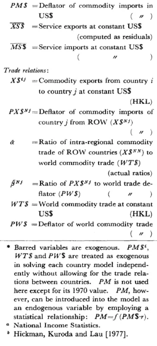
X$ = Commodity exports at constant

US$ (HKL)b

M$ =Commodity imports at constant

US$ ( " )

PX$ = Deflator of commodity exports in

"

PW$ =Deflator of world commodity trade (

"

) (HKL) US$

PM $ = Deflator of commodity imports in

US$ ( " )

XS $ =Service exports at constant US$ (computed as residuals)

MS$ =Service imports at constant US$

*

Barred variables are exogenous. PM $1., WT$ and PVV$ are treated as exogenous

in solving each country model independ-ently without allowing for the trade rela-tions between countries. PM is not used

here except for its 1970 value. PM,

how-ever, can be introduced into the model as an endogenous variable by employing a statistical relationship: PM=f(PM$·r). a National Income Statistics.

b Hickman, Kuroda and Lau [1977].

Trade relations:

X$1.j =Commodity exports from country i

to countryj at constantUS$ (HKL)

PX$Nj=Deflator of commodity imports of countryj from ROW (X$Nj)

(

"

a =Ratio of intra-regional commodity

trade of ROW countries(X$NN) to world commodity trade (Wr$)

(actual ratios)

pNj =Ratio ofPX$Nj to world trade de-flator (PW$) "

WT$ =World commodity trade at constant

( II )

1\1. EZ.AKI: Linking National Econometric l\;lodels

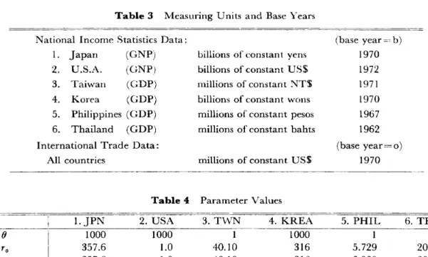
Table3 lVleasuring Units and Base Years

National Income Statistics Data:

1. Japan (GNP) billions of constant yens 2. U.S.A. (GNP) billions of constant US$ 3. Taiwan (GDP) millions of constant NT$ 4. Korea (GDP) billions of constant wons 5. Philippines (GDP) millions of constant pesos 6. Thailand (GDP) millions of constant bahts International Trade Data:

All countries millions of constant US$

(base year= b) 1970 1972 1971 1970 1967 1962 (base year= 0) 1970

Table 4 Parameter Values

I.JPN 2. USA 3.TWN 4. KREA 5. PHIL 6. THAI

() _{1000 1000 1 1000 1 1} To 357.6 1.0 40.10 316 5.729 20.93 Tb 357.6 1.0 40.10 316 3.900 20.84 PXo 1.000 9.31 .9744 1.000 1.757 1.016 PMo 1.000 .891 .9611 1.000 1.586 1.080 PYo 1.001 .9136 .9670 1.000 1.257 1.135 PM$b 1.000 1.121 1.037 1.000 .914 .870 PW$b 1.000 1.128 1.044 1.000 .924 .873 Yb 70613.3 1171.1 261558 2577.36 29515 63793

consideration, though there will be some minor changes in explanatory variables in the actual estimation.4) The country model here is quite similar to the model proposed by Klein and Van Peeterssen [1973] tentatively for France and Italy and can be characterized as the model of effective demand type since all of the behavioral equations for quantity vari-abies (C-4) .- (C-7) are specified as demand functions.

Equation (C-l) IS the GNP or GDP identity at constant prices in national income statistics (abbreviated as NIS). Equations (C-2) and (C-·3) are the identities at constant prices between the 4) The same is true for the trade model. In this sense, the model presented in Table 1 is called the prototype model.

NIS data in national currenCIes and the international trade data in US dollars, respectively for exports and imports of goods and services. As shown in Table 3, measuring units and base years are differ-ent not only from one country to another but also in NIS and international trade data. Therefore, appropriate adjustment factors (PXo/ro'8 and PMo/ro'()) must be

applied in the two accounting identities (See Table 4 for parameter values). In the present paper, the data for interna-tional commodity trade in US dollars are based exclusively on Hickman, Kuroda and Lau [1977]. As a result, the data for international servicetrade in US dollars XS$ and MS$) are derived as residuals by using the accounting identities (C-2) and (C-3).5) Equation (C-4) is the

con-sumption function of the usual type, where the oil shock dummy (nUM) is intro-duced when necessary, while equation (C-5) is the investment function of the simplest kind. Equations (C-6) and (C-7) are the demand functions for exports and imports, respectively, both of which are determined by the variables of the same nature. Note that in the case of import functions, measuring units and base years of the explanatory variables are adjusted to those of the dependent variables. By such an adjustment, the interpretation and comparison of the coefficient estimates will be made easier and more straightforward.6 ) Equation (C-8) assumes that the GNP deflator is determined by the levels of total demand (index of GNP) and import prices with the base year adjusted. Similarly, equa-tion (C-9) assumes that the export deflator for goods and services of the NIS base is determined by the levels of GNP deflator and world export prices with base year adjusted. The last equation (C-10) represents a statistical relationship be-tween the deflator for exports of goods and services and the deflator for com-modity exports.

Our country model, which consists of ten equations can be solved for ten

5) These identities are not the exact ones in terms of the actual data. Negative values are derived as residuals for several years on the imports of Taiwan and Korea and for one or two years on the imports of the Philippines and Thailand.

6) Such adjustment is unnecessary when the log-linear form is employed, since any kind of scale adjustment concentrates on the constant term in the actual estimation.

endogenous variables of each country if the data are given a priori to both of the predetermined variables (i.e., barred and lagged variables) and the three variables related to foreign countries or world market (WT$, PW$ and PlvI$i). This is the case of unlinked country model. The three world variables, however, must be determined in the world market by introducing trade relations among all of the countries in the world. As shown in Table 5, the world in the present paper is divided into six countries and the rest of the world (ROW), and our trade model (i.e., the linkage part of Table 1) describes the trade relations for these seven groups as well as for the entire world.

Equation (T-l) is the key equation for linkage. For the six countries except ROW, it specifies the exports from country i to countryj (X $iJ ) as a demand function of countryj, so that it may be called the import function of country j

for the exports of country i. The disa-ggregate import function (T-l) is derived on the basis of the same principle as the aggregate import function (C-7). How-ever, they are different in the treatment of relative prices which represent the price competitiveness in the market of im-porting country. In other words, the former (T-1) allows for the competl bve power of exporting country in the market of importing country in more details than the latter (C-7) by introducing two kinds of relative prices: PX$i/PM$J (i.e., com-petition with other countries exporting to country j) and PX$i·rJ/PYJ (i.e.,

M. EZAKI: Linking National Econometric Models

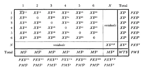
Table 5 Trade Relations with Particular Reference to the ROW Countries in the Link Model*

2 3 4 5 6 N Total 1 2 3 4 5 6 N Total X$ll X$12 X$13 X$14 X$15 X$16 X$l X$21 ₀ X$23 X$24 X$25 X$26 X$2 X$31 X$32 0 X$34 X$35 X$36 X$3 residuals X$41 X$42 X$43 0 X$45 X$46 X$' X$51 X$52 X$53 X$54 0 X$56 X$5 X$61 X$62 X$63 X$64 X$65 0 X$6 residuals I X$NN X$N M$l M$2 M$3 M$4 M$5 M$6 M$N WT$ PX$Nl PX$.Y2 PX$N3 PX$.\'4 PX$N5 PX$N6 PX$NN PM$l PM$2 PA-f$3 PAf$4 PM$5 PAI$6 PjW$N

PX$l PX$2 PX$3 PX$4 PX$5 PX$6 PW$

*

Note that the trade data here are based on Hickman, Kuroda and Lau [1977] where Ryukyu is treated as part of the Japanese territory throughout the postwar period though it had been under the rule ofD.S.A. until 1972. As a result, the diagonal element which corresponds to Japan (country 1) does not vanish before 1972 so that it is treated as exogenous in the model.

competition with the importing country). Equations (T-2) -- (T-8) are concerned about the ROW countries, for which nei ther export and import functions such as (C-6), (C-7) and (T-1), nor export price function such as (C-10) are specified explicitly. Instead, exports and imports of the ROW sector are determined as residuals by equations (T-2) and (T-3) as is illustrated in Table 5. Furthermore, the intra-regional trade (X$NN) and the export prices (PX$NJ'S) of the ROW countries are assumed to be proportional to total world trade (WT$) and world export price (PW$), respectively, by equations (T-4) and (T-5). The pro-portionality factors (a and (3's) are treated as exogenous and their data are the actual ratios, so that the introduction of equations (T-4) and (T-5) will be almost equivalent with the exogenous treatment of X$NN and PX$NJ.7) We

need, for the ROW sector, such devices as equations (T-4) and (T-5) in order to avoid misleading results in case of the policy simulations (See Section 4). That is to say,X$NN and PX$NJ are assumed to maintain their ratios to WT$ and PW$,

respectively, at the actual historical levels even when the data for policy variables in some country are changed to analyze the policy effects based on the simulation method. The three remaining equations (T-6) -- (T-8) are all concerned about the aggregate identities in quantity or price for the ROW countries taken as a whole.

Equations (T-9) and (T-10) are also the aggregate identities in quantity or

7) Concerning the world variables (WT$ and

PW$), the final test based on the former

shows slightly bigger deviations from actual values than the final test based on the latter. Note that the data for a are distributed be-tween 0.634 and 0.667 with a slightly down-ward trend.

price for the world as a whole. Note that total world trade (WT $) can be defined either from export side or from import side, since total exports (2X$) and total imports (IM$) are always identical in the present model. The last equation (T-11) defines the import price index for each country as well as for the ROW sector. Price indexes in the present paper are defined basically as implicit deflators (such as equations (T-8) , (T-IO) and (T-11 ) ), so that the world identi ty be-tween total exports and total imports is valid not only in terms of quantity (i.e.,

IX$=IM$) but also in terms of value

(i.e.,2PX$,X$=2PM$·M$).

Unlike the system of Project LINK,S) our prototype model for linkage deter-mines the imports of ROW sector from other countries (X SiN) as residuals by equation (T-3) without suppressing the export function (C-6) of each country.

It may be possible, however, to introduce explicitly the import functions of ROW countries based on the principles similar to equation (T-I), and to replace the ag-gregateexport function (C-6) by the sum of component exports in each country. Similarly, for the exports of ROW sector to other countries (X$NJ), it is possible (and easier than the case of the imports of ROW sector above) to introduce the import functions of each country from ROW, and to replace the aggregate import function

(C-7)

by the sum of component imports in each country.

8) See Gana, Hickman and Lau [1977], which gives a good summary of various linking methods employed in Project LINK.

Our prototype model for linkage may be modified in this direction on the treatment of ROW sector. However, the present model does not seem to be inferior to the possible modified version, unless we suc-ceed in developing a model for the ROW sector which can explain the import .behavior of the sector well.

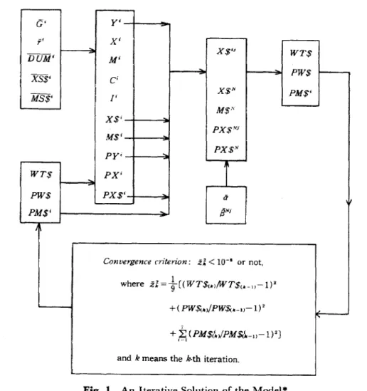
Our model for linkage is a system of non-linear equations for which some iterative procedure is unavoidable to get the solution. Figure I illustrates an iter-ative method which is adopted in the present paper.9) Note that the country model here is essentially a linear system,

i.e., linear in endogenous variables, if the data for WT$, PW$ and PM$£ are fixed

a priori, since PM $'rjPYin equation (C-7) is reversed into PYjPM$'r in the actual estimation. Therefore, the solution for ten endogenous variables in the country model can easily be obtained for each country under the given WT$,PW$ and

PM$£. When the data for WT$, PW$

and PM$£ are set equal to their actual values which are the initial values of our iterative process, we get the solution for the unlinked country model, with which the first iteration starts. (See the upper-left part of Figure I). The solution of the unlinked country model is used to compute the left-hand side variables of the trade model (i.e., equations (T-I)-(T-11», the last three of which are again

WT$, PW$

and

PM$£.

(See the upper-right part of Figure I). The new data

9) It is similar to the iterative method employed in Klein and Van Peeterssen [1973] (Fig. 4, p.454).

M. EZ.AKI: Linking National Econometric Models C' y' if _X' DUM' M' X$'i WT$ PW$ I -XS$' C' MS$' X$N _PM$' /' M$" X$' M$' PX$Ni py' PX$'V WT$ PX'

i

PW$ PX$' a _1/ PM$'

e

Ni

Convergence cn'tenon: zl<10-1 _{or not,}

where zl=~ [(WT$(>l(tVT$(._Il-l)'

+(PW$.,!PW$.-ll-l)'

+

±

(PM$(~>!PM$r.~-ll-l)2J

1-"l

andkmeans the k-th iteration,

Fig. 1 An Iterative Solution of the Model.

·WT$, PW$ and PM$J are exogenous in the case of unlinked country model, i.e., in solving each country model independently without allowing for the trade relations between countries, The three variables become endogenous in solving the whole linked system.

for WT$, PW$ and PM$' thus obtained give a new solution for the country model, with which the second iteration starts. This iterative process continues until the

convergence criterion shown in Figure 1 is satisfied, and we get the solution for the whole linked system.

III EstiJnation and Simulatability of the Model

The OLS method is applied in the present study to the prototype model of Table I or its variations. The estimation period is 1961-1975 for the five countries except for Korea.I°) The NIS data 10

Korea are available only from 1962 so

10) The international trade data by Hickman, Kuroda and Lau [1977] are available for 1955-1975. The NIS data ofJapan, U.S.A. and Taiwan are available from the biginning of the 1950's until recently, while those of the Philippines and Thailand are available for 1960-1975.

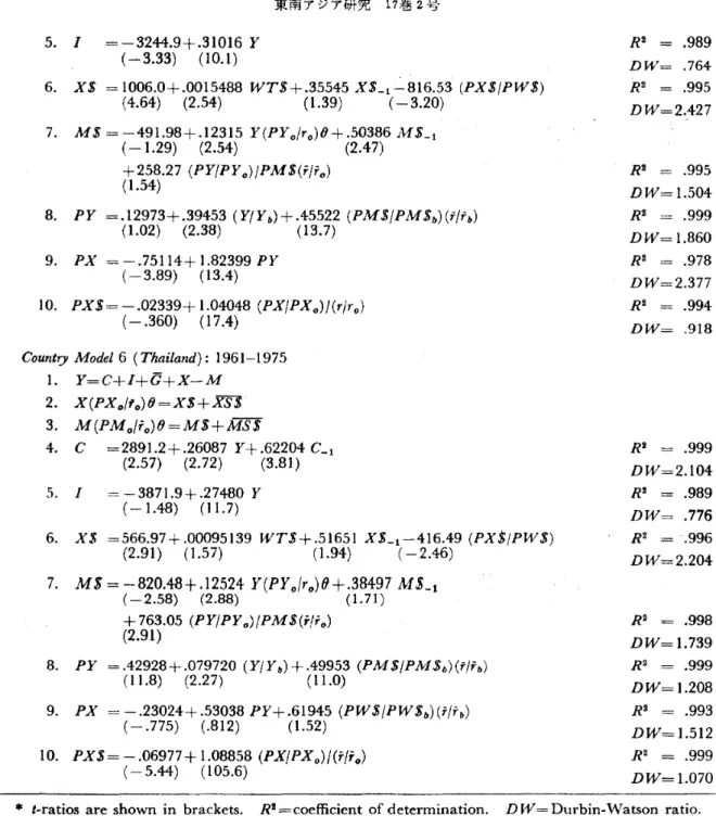
that the Korean country model and import functions are estimated for the period 1963-1975 with due allowance for lagged variables. As a result, the sim-u1atability of our linked system is checked for the period 1963-1975. The results of

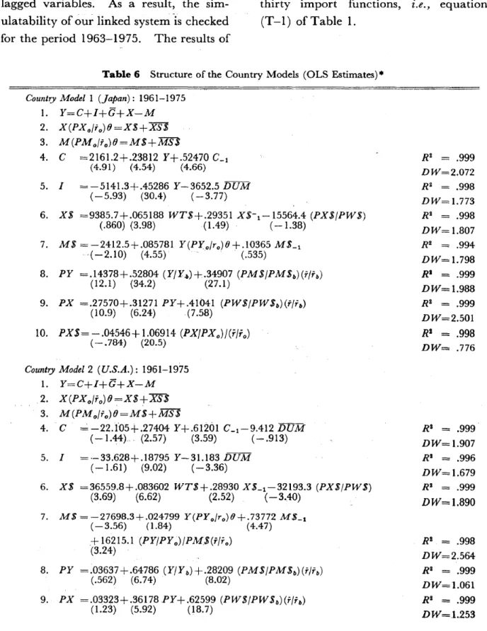
estimation are presented in Table 6 for the country model of six countries and in Table 7 for the trade model consisting of thirty import functions, i.e., equation (T-I) of Table 1.

Table 6 Structure of the Country Models (OLS Estimates)*

Country Modell (Japan): 1961-1975

1. Y=C+I+G+X-M 2. X(PXo/io)O=XS+XS$ 3. M(PMo/fo)O=M$+MS$ 4. C =2161.2+.23812 Y+.52470 C_1 (4.91) (4.54) (4.66) 5. I =-5141.3+045286 Y-3652.5 DUM (-5.93) (3004) (-3.77) 6. XS =9385.7+.065188 WTS+.29351 XS-1-15564A (PX$/PWS) (.860) (3.98) (1.49) (-1.38) 7. MS= -2412.5+ .085781 Y(PYo/ro)O + .10365 MS_1 ~(-2.1O) (4.55) . . (.535) 8. PY =.14378+.52804 (Y/Y,b)+.34907 (PMS/PMSb)(i/f b) (12.1) (34.2) (27.1) 9. PX =.27570+.31271 PY+AI041 (PWS/PWSb)(f/ib) (10.9) (6.24) (7.58) 10. PX$= - .04546+ 1.06914 (PX/PXo)/(r!io) (-.784) (20.5)

Country Model 2(U.S.A.): 1961-1975

1. Y=C+I+G+X-M

2. X(PXo/io)O=XS+XS$

3. M(PMo/fo)O=MS+MS$

4.

c

~-22.1'05+.27404 Y+.61201 C_1-9AI2 DUM

(-1.44).. (2.57) (3.59) (- .913) 5. I = ·-33.628+.18795 Y-31.183 DUM (-1.61) (9.02) (- 3.36) 6. XS =36559.8+.083602 WTS +.28930 XS_1-32193.3 (PXS/PWS) (3.69) (6.62) (2.52) (-3.40) 7. M$= -27698.3+.024799 Y(PYo!ro)f)+.73772 M$_l (-3.56) (1.84) (4047)

+

16215.1 (PY/PYo)/PM$(f/f0) (3.24) 8. PY =.03637+.64786 (Y/Y b) +.28209 (PMS/PMS,,)(i/f b) (.562) (6.74) (8.02) 9. PX =.03323+.36178PY+.62599 (PWS/PWSb)(f/i,,) (1.23) (5.92) (18.7) RI

=

.999 DW=2.072 R2 = .998 DW=1.773 R2 = .998 DW=1.807 R2 = .994 DW=1.798 RI = .999 DW=1.988 RI = .999 DW=2.501 RB

=

.998 DW= .776 RI = .999 DW=1.907 RI = .996 DW=I.679 RI = .999 DW=1.890 R2 = .998 DW=2.564 R2 = .999 DW=1.061 R2

=

.999 DW=1.253

M. EZAKI: Linking National Econometric Models Table 6 (continued)

10. PXS=-.00798+ 1.00150 _{(PX/PXo)/(f/fo)} (-1.23) (166.1)

Count~yModel 3 (Taiwan): 1961-1975

1. Y=C+I+G+X-M 2. X(PXo/fo)fJ=XS+XS$ 3. M(PMo/io)(}=MS+MS$ 4. C = 10148.6+ .30915 Y + .38737 C_1 (5.47) (5.76) (3.36) 5; 1 = -23802.9+.35345 Y (-4.69) (15.7) 6. X$ = -28.064+.0040352 WT$+.87673 X$_t-687.07 PX$ (-.071) (2.69) (4.97) (-2.65)

7. JvI$ = -287.15+.31451 _{Y(PY o!ro})fJ+.54402 JvI$_t-518.69 PM$(T/fo )

(-.549) (2.97) (1.48) (-1.04) 8. PY =.03387+.28897 _{(Y/Y b)+.66266 (PM$/P.M$b)(i/f b)} (1.26) (6.11) (14.9) 9. PX =.15139+.29142 PY+.58553 (PW$/PWSb)(f/rb) (2.92) (1.21) (2.54) 10. PX$=.05011+.97130 (PX/PXo)!U!i o) (.565) (12.4)

Countr:y Model 4 (Korea): 1963-1975

1. I'=C+I+G+X-M 2. X(PXo!fo)f}=X$+XS$ 3. M(PMo/fo)fJ=M$+MS$ 4: C =38.734+.18744 Y+.78309 C_t-115.15 DUM (.745) (1.69) (4.10) (-3.58) 5. I = -225.85+.33148 Y· (-3.72) (14.4) 6. XS =462.57+.0040811 WT$+.74861 X$_t-1268.9 (PX$/PW$) (.564) (2.66) (3.92) (-1.36)

7. M$ =-1159.4+.32393 Y(PY o/ro)fJ+480.42 (PY/PYo)/PM$(iFo)

(-2.51) (15.7) (1.02) 8. PI' 0--==-.24856+1.05279 (I'/Yll)+.19063 (PM$(PM$b)(f/rb) (02.55) (5.44) (2.17) 9. PX =~.29912+.25451PI'+.46809 (PW$/PWS1i)(f/fb) (9.87) (2.76) (7.81) 10. PXS=-.07561+1.03456 (PX/PXo)/(r(ro) ( - .266) (4.03)

Country Model 5 (Philippines): 1961-1975

1. Y=C+I+G+X-M 2. X(PXo/fo)(}=X$+XS$ 3. M(PMo/fo)(}=M$+MS$ . 4. C =691.15+.D84134 Y+.89105C-1 (1.32) (.750)" (5.07) R3 = 1.000 DW=I.593 R3 = .999 DW=I.830 R2 = .988 DW=2.192 R2 = .995 DW=1.368 R2 = .994 DW=1.927 R2 = .999 DW= .993 R'l. = .998 DW=1.867 RZ = .994 DW= 1.635 R'l. = .999 DW= 1.325 R2 = .989 DW= 1.208 R2 ~ .992 DW=2.752 R2 = .992 DW= 1.687 R2 = .995 DW=1.742 R2 = .999 DW= 1.857 R2 = .981 DW= .993 R" = .999 DW~·1.996

5. I = -3244.9+.31016 Y

(-3.33) (10.1)

6. X$ = 1006.0+.0015488 WT$+.35545 X$_1-816.53 (PX$/PW$)

(4.64) (2.54) (1.39) (-3.20)

7. M$ =-491.98+.12315 Y(PY o/ro)8+.50386Af$_l

(-1.29) (2.54) (2.47) +258.27 (PY/PYo)/PM$(r/ro) (1.54) 8. PY =.12973+.39453 (Y/Y b)+.45522 (PM$/PM$b)(r/f_b) (1.02) (2.38) (13.7) 9. PX = -.75114+ 1.82399 PY (-3.89) (13.4) 10. PX$= -.02339+ 1.04048 (PX/PXo)/(r/ro) (-.360) (17.4)

Country Model6 (Thailand): 1961-1975

1. Y=C+I+G+X-M 2. X(PX o/fo)8=X$+XS$ 3. M(PMo/'o)()=M$+MS$ 4. C =2891.2+.26087 Y+.62204 C_1 (2.57) (2.72) (3.81) 5. I =-3871.9+.27480 Y (-1.48) (11.7) 6. X$ =566.97+.00095139 WT$+.51651 X$_1-416.49 (PXS/PW$) (2.91) (1.57) (1.94) (-2.46) 7. MS=-820.48+.l2524 Y(PYo

lr

o)O+.38497 M$_l (-2.58) (2.88) (1.71) +763.05 (PY/PYo)/PM$(i!ro) (2.91) 8. PY =.42928+.079720 (Y/Y b) +.49953 (PM$/PM$b)(f/fb ) (11.8) (2.27) (11.0) 9. PX = -.23024+.53038 PY+.61945 (PW$/PW$b)(f/fb ) (- .775) (.812) (1.52) 10. PX$= -.06977+ 1.08858 (PX/PXo)/(i"/io) ( - 5.44) (105.6) R2 = .989 DW= .764 R2 = .995 DW=2.427 R2 = .995 DW=1.504 R2 = .999 DW=1.860 R2 = .978 DW=2.377 R2 = .994 DW= .918 R2 = .999 DW=2.104 R2 = .989 DW= .776 R2 = .996 DW=2.204 R2 = .998 DW=1.739 R2 = .999 DW=1.208 R2 = .993 DW=1.512 R2 = .999 DW=I.070

* t-ratios are shown in brackets. R2=coefficient of determination. DW=Durbin-Watson ratio.

Table 7 Structure of the Trade Model (OLS Estimates): 1961-1975*

X$iJ _CONST Y$J X$~{ PX$i/PM$J PX$i/PY$J PX$i(rJ/rt) R2

DW USA- 3210.1 .020826 -3168.6 .989 JPN (1.89) (8.73) ( -2.00) 1.994 TWN- -95.301 .0014902 .35942 .954 JPN (-1.71) (2.95) (1.69) 1.710 KREA- 210.64 .0033074 .26094 -598.97 .937 JPN (.569) (3.00) (.830) ( -1.32) 2.103 PHIL- 219.20 .0015072 -127.47 .992 JPN (2.51) (8.27) (- 1.92) 2.369

M. EZAKI: Linking l'\ational Econometric Models THAI- -10.511 .00058248 .51616 .994 JPN (- .875) (2.58) (2.40) 1.939 JPN- 1385.6 .0038361 .73816 -3132.7 .992 USA (.496) (L 11) (3.61) ( -2.66) 2.770 TWN- -59.565 .00056305 .87066 -299.60 .986 USA (- .165) ( 1.56) (7.37) ( -2.29) 1.009 KREA- - 261.69 .0013645 .48555 -659.83 -170.85 .997 USA (-1.71) (2.82) ( 1.89) ( -1.87) ( -1.49) 2.634 PHIL- 169.34 .0000277 .76105 -83.998 .993 USA (2.15) (.164) (1.91 ) ( -1.46) 1.625 THAI- 92.101 .00012011 .24285 -113.14 -16.406 .980 USA (.986) (1.97) (1.17) (- 1.56) (-.631) 1.904 JPN- 29.163 .12960 .57884 -386.93 .996 TvVN (.198) (3.18) (2.43) (- 3.83) 2.516 USA- 1144.5 .10275 -1253.1 .990 TWN (2.89) (9.97) ( -3.29) 2.356 KREA- 12.229 .0043326 .31394 -27.366 .958 TWN (.988) (3.24) (1.12) (-1.91) 2.305 PHIL- 10.284 .0036103 .25334 -15.804 .960 TWN (3.13 ) (4.05) (1.15) (- 3.58) 2.478 THAI- -16.498 .0076884 .891 TWN ( -2.22) (5.64) 2.449 JPN- 3143.2 .11434 -3088.5 -165.80 .993 KREA (3.24) (10.4) ( -3.54) (- 1.36) 1.940 USA- 813.71 .076625 -505.29 -266.66 .993 KREA (1.61 ) (10.6) ( -1.24) ( -1.97) 2.050 T\VN- -28.075 .0073928 .939 KREA (- 3.44) (7.58) 2.393 PHIL- 9.0582 .0029607 -11.576 .894 KREA ( 1.29) (2.15) (-2.50) 1.067 THAI- -2.7504 .0005176 1.00100 .962 KREA (- 1.58) ( 1.88} (4.83) 2.263 JPN- 983.35 .10292 .36343 -1223.8 -218.32 .997 PHIL (2.89) (4.38) (2.79) ( -3.86) ( -4.48) 1.785 USA- 734.71 .015308 .33982 -361.79 -260.83 .994 PHIL (2.76) ( 1.02) (1.44) ( -1.58) ( -1.99) 2.012 TWN- -12.308 .0042338 .72606 -11.103 .940 PHIL (-.899) ( 1.44) (1.16) (- 1.32) 1.344 KREA- 2.0986 .0010676 -7.4457 .923 PHIL (.705) (5.63) ( -2.93) 2.179 THAI- 8.1990 .0033712 -20.358 .737 PHIL (.760) (1. 72) ( -1.40) 1.322 JPN- 372.71 .055966 .30930 -429.55 .999 THAI (4.63) (4.06) (1.80) ( -4.47) 2.256 USA- 401.07 .014912 .24435 -137.50 -244.94 .984 THAI (1.09) (2.21) (.964) ( -1.00) ( -1.50) 2.202 TWN- 4.9397 .0058414 -12.502 .986 THAI (.706) (l0.8) ( -1.90) 1.486 KREA- .61501 .0015976 .29520 -5.8570 .936 THAI (.071 ) (2.65) (.962) ( -.588) 1.911 PHIL- 2.1872 .0003950 .47451 -3.6962 .888 THAI (1.51 ) (2.21 ) (1.94) ( -2.27) 1.744

• Korean imports (X$i4) : 1963-1975. i-ratios are shown iQ brackets. Y$J= Yj(PY~/rt)()J and

The country models of Table 6 are derived after many trials and errors for each equation. Since the prototype model in Table I incorporates and allows for the results of such trials and errors, it may be said to be dependent also on the actual country models adopted here. In any case, the actual country models are basically the same as that of the pro-totype model. However, some minor differences or changes in explanatory variables between them are inevitable judging from signs and significance levels of the estimated coefficients,

R2

and the Durbin-Watson ratios. For example, in the import function of Japan (eq. 7), the price variable is dropped.H ) In the export and import functions of Taiwan (eqs. 6 and 7), the absolute price levels are introduced in place of the relative price levels. 1n the import function of Korea (eq. ,7), the lagged variable is excluded. In the export price function of the PhiIlppines (eq.

9),

the world export price is dropped by reason of wrong sign, which seems serious so that the equation must be improved in some way or other. Finally, in the export price function of Thailand (eq. 9), the GDP deflator is not significant enough. !vIost of these changes and reservations are of minor importance. Our prototype model may be said to summarize well the common and basic features of individual countries.

11) Note that the lagged vanable is not significant though it is included in the equation. We get similar. results .also based, on" the NTS ,data." which is,different in the treatnlentof Ryukyu from the present data.

17~2

'5-This is true especially for the US case In which the actual country model coincides completely with that of the prototype model.

The actual trade model of Table 7 is also based on the results derived after many trials and errors for each equation. The present model has a merit in esti-mating individual import functions in-dependently on the country-by-country basis without using such devices as trade share matrix. As a result, we have thirty import functions which are esti-mated independently as the demand functions of each importing country,

i.e.,

five for each of the six countries. As in the case of country model, the actual trade model (i.e., import functions) shown in Table' 7 deviates more or less from that of the prototype model. The deviations occur mainly in relation to the treatment of price variables.l2) The case is quite rare where both of the two relative prices

(PX$i/PM$J and PX$i/PY$J) must be introduced to distinguish between two kinds of price competitiveness in the market of importing country. Actually, the competition of an exporting country with domestic suppliers (PX$t/PY$J) is far more important in explaining import behaviors than the competition of an exporting country with other foreign suppliers (PX$t/PM$J). In some cases, especially for Taiwan, the absolute price

12) In the case of Korean imports, the lagged variable is mostly of wrong sign or insignifi-cant. Even when it is introduced as an effec-tive explanatory' factor- (i.e.,THAI-KREA), it gives a rather extraordinary estimate of coefficient which is greater than one.

I\'1. EZAKI: Linking National Econometric .Models

level (PX $£'rJ ) turns out to be more significant than the relative price levels.I3 )

The explanatory variables here are se-lected, of course, based on the signs and t-ratios of coefficient estimates (as well as on R2 and the Durbin-Watson ratios). The result of selection for price variables in Table 7 seems to reflect, to some extent, the comodity composition of imports in each country, since exports and im-ports in the present study are treated only in total. The same may be true for the other two explanatory variables (Y$J and

X$~l)' especially for the latter. For the income variable (Y$J), however, the co-efficient estimates are always positive and highly significant with only one exception,

i.e., the case of PHIL-USA. The income variable may be said to be tIl(' most impor~ant and universal factor of ex-planation in the import functions of any kind for any country.

When the structure is specified for both coun try and trade models as shown in

Tables 6 and 7, we can solve the linked system by the iterative method illustrated in Figure 1 for each year to test the simulatability of the model. The sim-ulatability is usually checked by the dynamic simulation (called final test), which means to solve the model for each year using estimated values (not actual ones) for lagged endogenous variables. The final test in graphical form, which is ami tted to save space (See Ezaki [1978J, Fig. 2, pp. 20-26), shows that our linked system can simulate the actual economy to a remarkable extent not only for each country but also for the ROW sector and the entire world.14 ) The simulatability of t he present linked system seems to be adequate enough to be used for various policy simulations. Not to mention, the final test for the unlinked country model is better than that of the linked system because the three world variables are treated as exogenous in the former.

IV Policy Shnulations

The model of the present paper contains two policy variables: the government consumption expenditures at constant prIces (G£'s) and the exchange rates

(ri's). The dynamic simulations are

13) The same was true for the aggregate import function of Taiwan (See Table 6). In the case of Philippine imports from Japan (i.e .. JPN.PHIL), both of the relative and absolute prices are introduced because of their good statistical propertit:s, though it is difficult to give good economic interpretations to the equation.

applied here to the unlinked country model as well as to the linked system for 14) In some cases, irnports of the country-by-country basis (X$£J) have strong cyclical clements. which are not traced well by the present model. In the case of Korean total exports (X$),the simulated values are nega-tive for 1963 and 1964. This is due to the fact that Korean exports increased extremely rapidly from a quite low level in 1963 or 1964. Note that the number of iterations, which corresponds to· the convergence criterion of Figure 1, varies from year to year: 25-40 for 1963-1970, and 50-60 for 1971-1975.:

*TtO" :/7"*~ 17~2 f}

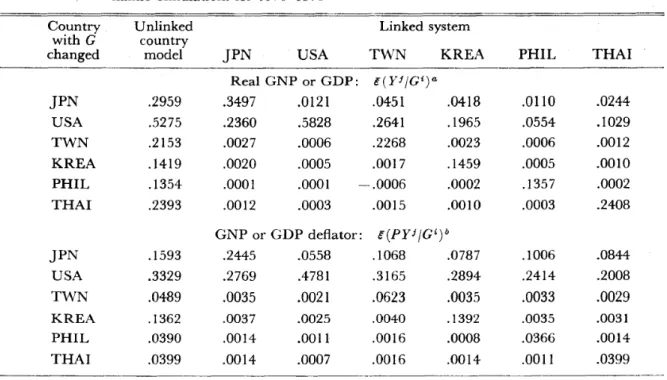
Table 8 Elasticities of Government Expenditures: Average Figures Based on the

Dy-namic Simulations for 1971-1975*

Country Unlinked Linked system

with G country

changed model JPN USA TWN KREA PHIL THAI

Real GNP or GDP: e(YfIGi)a JPN .2959 .3497 .0121 .0451 .0418 .0110 .0244 USA .5275 .2360 .5828 .2641 .1965 .0554 .1029 TWN .2153 .0027 .0006 .2268 .0023 .0006 .0012 KREA .1419 .0020 .0005 .0017 .1459 .0005 .0010 PHIL .1354 .0001 .0001 -.0006 .0002 .1357 .0002 THAI .2393 .0012 .0003 .0015 .0010 .0003 .2408

GNP or GDP deflator: e(PYf jGi)b

JPN .1593 .2445 .0558 .1068 .0787 .1006 .0844 USA .3329 .2769 .4781 .3165 .2894 .2414 .2008 TWN .0489 .0035 .0021 .0623 .0035 .0033 .0029 KREA .1362 .0037 .0025 .0040 .1392 .0035 .0031 PHIL .0390 .0014 .0011 .0016 .0008 .0366 .0014 THAI .0399 .0014 .0007 .0016 .0014 .0011 .0399

• Computed at the point where G (real) is changed by

+

10% for each country throughout h . I ' . d ' 4GijGi 0 l(i=JPN, ,THAI) I h f l' k d t e Simu atlOn peno ,I.e., ~ t t= . t=1971, , 1975 . n t e case0 un In e

coun-try model, change in G in certain country does not influence economic activities of other countries so that only the own elasticities (i.e., diagonal elements) arc shown above.

a e(YfjGi)==(.1yfj.1Gi)'(Gijyf),

where Gi=actualGi, averaged for 1971-75 (i.e., (ljS)l'GD, .1Gi=change inGi,

Yf=simulated yf under unchanged Gi, averaged for 1971-75,

.11'"f+ yf= simulated yf under changedGi, averaged for 1971-75.

b e(PYf IGi)

==

(.1PYf I ilGi)·(GiIPYf),

where pyf=(simulatedpyf.yf,averaged)j(simulated yf, averaged), under unchanged G, JPYf+PYf=(simulatedPYf·Yf, averaged)I(simulated yf, averaged), under changedG.

the period 1971-1975 to quantify the effects of the changes in these policy variables in that period.l5 ) The results are summarized in terms of average elasticities in Tables 8 and 9 for only two variables: GNP or GDP (Y) and its deflator (PY). The elasticity is a con-venient measure to see the effects on

15) We get similar results even when the simu-lation analyses are applied for the period 1966-1970.

prices, but the multiplier may be better if we want to compare the effects on quantities or values between countries. Tables 9 and 10 summarize the results of simulation in terms of average multipliers for several quantity or value variables. Definitions and computational procedures are explained in detail in each of the four tables. However, it should be stressed In the case of multipliers that the measuring unit for quantities or values in

1'\'1. EZAKI: Linking National Econometric J\lodels

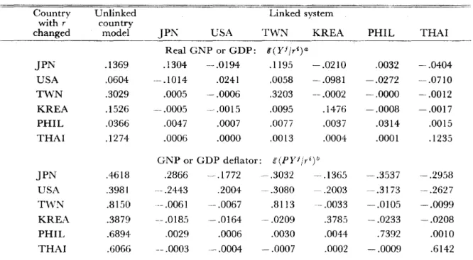
Table 9 Elasticities of Exchange Rates: Average Figures Based on the Dynamic Simu-lations for 1971--1975*

Country Unlinked Linked system

with r country

changed model JPK USA TWN KREA PHIL THAI

Real GNP or GDP: e(YJjri)a JPN .1369 .1304 -.0194 .1195 -.0210 .0032 -.0404 USA .0604 ---.1014 .0241 .0058 -.0981 -.0272 -.0710 TWN .3029 .0005 -.0006 .3203 --.0002 -.0000 - .0012 KREA .1526 --.0005 -.0015 .0095 .1476 -.0008 - .0017 PHIL .0366 .0047 .0007 .0077 .0037 .0314 .0015 THAI .1274 .0006 .0000 .0013 .0004 .0001 .1235

GNP or GDP deflator: e(PYJ /ri)b

JPN .4618 .2866 -.1772 -.3032 -- .1365 -.3537 -.2958 USA .3981 -- .2443 .2004 ~.3080 - .2003 -.3173 -.2627 TWN .8150 --.0061 -- .0067 .8113 -- .0033 -.0105 -.0099 KREA .3879 -- .0185 -.0164 -.0209 .3785 -.0233 -.0208 PHIL .6894 .0029 .0006 .0030 .0044 .7392 .0010 THAI .6066 -- .0003 -.0004 -.0007 .0002 -.0009 .6142

* Computed at the point where ris changed by

+

10% (i.e., devaluation) for each country throughout the simulation period, i.e.,

JrUr~=O.1 (i=JPN, ... ,THAI; t= 1971, ... ,1975).

Note that the 10% devaluation of US exchange rate (from 1.0 to 1.1) means the devaluation of US dollars to every country. \Vhen r is changed for each country by - 10% (i.e., ap-preciation), almost the similar results (different by 10-20% in absolute value) are obtained with the signs almost completely opposite. In the case of unlinked country model, again, change in r in certain country does not affect economic activities of other countries.

a e(YJ/ri)=(LlYJ/Jri)'(i.i/yr). See footnote ato Table 8.

b !(PYi/r i )

=-

(JpyJ/ dri)'(fi/pyJ). See footnote b to Table 8.

each country is standardized (i.e.-, con-verted into US dollars) to make the international companson direct. Note that, in the case of unlinked country model, the change in G or r in a certain country does not affect economic ac-tivities of other countries by the pro-perites of the model. In Tables 8~11, therefore, are shown only the own elasticities or own multipliers for the unlinked country model, which must be compared with the diagonal elements of elasticity or multiplier matrices for the

linked system.

Let us begin with the case where the government consumption expenditures at constant prices are changed in each of the

SIX countries respectively. From the

simulation results summarized in Tables 8 and 10, we can derive basic facts and implications which underlie the inter-dependent relations among countries, and clarify the advantages and merits of the linked system compared to the unlinked country model.

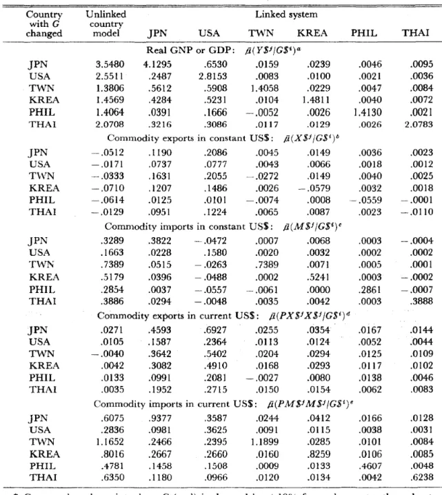
Table 10 Multipliers of Government Expenditures: Average Figures Based on the Dy-namic Simulations for 1971-1975*

Country Unlinked Linked system

with G country

changed model JPN USA TWN KREA PHIL THAI

Real GNP or GDP: il(YS1jGSi)a JPN 3.5480 4.1295 .6530 .0159 .0239 .0046 .0095 USA 2.5511 .2487 2.8153 .0083 .0100 .0021 .0036 TWN 1.3806 .5612 .5908 1.4058 .0229 .0047 .0084 KREA 1.4569 .4284 .5231 .0104 1.4811 .0040 .0072 PHIL 1.4064 .0391 .1666 -.0052 .0026 1.4130 .0021 THAI 2.0708 .3216 .3086 .0117 .0129 .0026 2.0783

Commodity exports in constant US$: j1(XS1jGSi)b

JPN -.0512 .1190 .2086 .0045 .0149 .0036 .0023 USA -.0171 .0737 .0777 .0043 .0066 .0018 .0012 T\VN -.0333 .1631 .2055 -.0272 .0149 .0040 .0025 KREA -.0710 .1207 .1486 .0026 - .0579 .0032 .0018 PHIL -.0614 .0125 .0101 -.0074 .0008 -.0559 - .0001 THAI -.0129 .0951 .1224 .0065 .0087 .0023 -.0110

Commodity imports in constant US$: j1(M$1jG$i)C

JPN .3289 .3822 -.0472 .0007 .0068 .0003 -.0004 USA .1663 .0228 .1580 .0020 .0032 .0002 .0002 TWN .7389 .0515 - .0263 .7389 .0071 .0005 .0001 KREA .5179 .0396 -.0488 .0002 .5241 .0003 -.0002 PHIL .2854 .0037 - .0557 -- .0061 .0000 .2861 -.0007 THAI .3886 .0294 -.0048 .0035 .0042 .0003 .3888

Commodity exports in current US$: il(PX$1X S1 JGSt)d

JPN .0271 .4593 .6927 .0255 .0354 .0167 .0144 USA .0105 .1587 .2364 .0113 .0124 .0052 .0044 TWN -.0040 .3642 .5402 .0204 .0294 .0125 .0109 KREA .0042 .3082 .4910 .0168 .0293 .0117 .0102 PHIL .0133 .0991 .2081 -.0027 .0080 .0138 .0046 THAI .0035 .1952 .2715 .0150 .0154 .0062 .0083

Commodity imports in current US$: il(PMS1M $1jG$i)e

JPN .6075 .9377 .3587 .0244 .0412 .0166 .0128 USA .2836 .0981 .3625 .0091 .0115 .0038 .0031 TWN 1.1652 .2466 .2395 1.1899 .0285 .0101 .0084 KREA .8016 .2667 .2660 .0160 .8259 .0106 .0085 PHIL .4781 .1458 .1508 .0009 .0133 .4607 .0048 THAI .6350 .1180 .0966 .0120 .0134 .0042 .6238

*

Computed at the point where G (real) is changed by

+

10% for each country throughout the simulation period. See footnotes to Table 8.

a il(Y$J /GSi)=E(YJ IGt).(Y$l /GSi)=J YSJ / JlJ$l,

where Y$J= Y1(PY

t/

rt)81 (i.e., in millions of constant 1970US$),

G$i=Gi(PG~Jr~)Oi (i.e., in millions of constant 1970US$),

l(Y1 /Gi)=(J Y1/ JGi).(Gi / y1)=(Jy$J /J{J$i).(GSi / YS1).

b /l(X$J IG$i)=l(X$J IGi).(nJ(efi )=

Jft

JI J(J$i).

e /I(MSJ /GSi)=l{MSi /Gi).(M$i/G$i) = JM$J I J{J$i.

d il(PXSJXSi IG$i)

=

l(PX$JX$J/Gi). (PX$1X$1 IGSi)= J(PX$JX$J)/ JGIi.

M. EZAKI: Linking National Econometric Models

Table 11 Multipliers of Exchange Rates: Average Figures Based on the Dynamic

Simu-lations for 1971-·1975* Linked system Country with r changed Unlinked country

model JPN USA TWN KREA PHIL THAI

Real GNP or GDP: p(Y$Jjri)jlooa JPN 326.52 306.91 -208.78 8.38 ~-2.39 0.26 -3.14 USA 652.09 - 238.48 259.71 0.41 -11.17 -2.28 -5.52 TWN 21.98 1.10 -6.31 22.46 -0.03 -0.00 -0.09 KREA 17.55 -1.05 -15.90 0.67 16.80 -0.07 -0.21 PHIL 3.07 10.95 7.61 0.54 0.42 2.62 0.12 THAI 9.93 1.39 0.41 0.09 0.05 0.01 9 ..19

Commodity exports in constant US$: /1(X $f /ri) j 100b

JPN 84.10 82.65 10.92 11.86 0.26 1.02 0.78 USA 80.31 -63.51 8.87 5.57 -5.94 -1.39 -0.58 TWN 3.73 0.60 1.24 4.14 0.05 0.02 0.03 KREA 8.38 0.10 0.96 0.86 8.07 -- 0.02 0.04 PHIL 1.41 3.18 4.21 0.39 0.30 1.00 0.06 THAI 0.39 0.43 0.59 0.09 0.04 0.01 0.37

Commodity imports in constant US$: p(M$f /r i )j100"

JPN 30.41 28.45 78.73 9.62 0.69 0.70 1.55 USA -141.58 -22.13 -- 78.08 5.32 -2.61 0.15 0.81 TWN -1.28 0.09 2.99 -0.94 0.03 0.02 0.05 KREA 3.39 -0.11 6.11 0.67 3.23 0.02 0.09 PHIL -0.57 1.01 1.05 0.26 0.15 -0.65 0.03 THAI -2.02 0.13 0.32 0.06 0.02 0.00 -2.01

Commodity exports in current US$: P(PX$1X $f jr i )/ 100d

JPN -34.34 --120.94 -229.16 6.19 -8.32 -6.36 -5.34 USA -42.07 --201.27 -397.71 -4.05 -17.00 -8.98 -7.80 TWN 0.30 -2.27 -7.01 0.91 --0.24 --0.19 -0.17 KREA 0.52 -8.53 -20.59 0.37 -0.27 -0.53 -0.48 PHIL -0.29 5.52 6.69 0.65 0.45 0.17 0.13 THAI -0.07 0.43 0.14 0.10 0.03 -0.00 -0.04

Commodity imports in current US$: P(PM $f M $J/rt) j 100e

JPN 53.34 -85.02 -186.59 --2.06 -20.98 - 10.97 -7.70 USA -221.93 -·200.50 -407.19 .- 7.31 -22.98 ~--]0.33 -7.5] TWN -1.73 -5.31 -6.99 - 1.39 --0.57 -0.33 -0.25 KREA 5.66 - ]5.90 -18.59 -0.09 4.44 -0.74 -0.55 PHIL -0.81 2.07 1.79 0.46 0.29 0.60 0.06 THAI -2.78 -0.29 -0.36 0.05 -0.01 -0.02 --2.57

* Computed at the point where r is changed by

+

10% (i.e., devaluation) for each country throughout the simulation period. See footnotes to Table 9. Note that multipliers are all divided by 100 so that they indicate the effects (in million $) of the 1% change in r.

a p(Y$f/ri)=.e(Y1/ri).Y$1=JY$f/(J:rijii) (in millions of constant 1970US$)

b P(X$f Iri)=.e(X$f Ir i ).X$1= JX$1 I(Jfijti (in millions of constant 1970 US$) c p(M$1 Ir i ) =.e(M$1 Ir i ).M$1

=

11M$i I (11fi If i ) (in millions of constant 1970 US$) d p(PX$1X$f Ir i ) =e(PX$1 X$f Iri).PX$f X$1

=

11(PX$f X$J)/(Jf i

rr

i)

(in millions of current US$)

e P(PM$1M$1 Iri)=.e(PM$j M$f Ir i ).PM$1M$1

=

J(PM$JM$J)/(Jft1ft )

16) Note that, when the off-diagonal elements are divided by the diagonal elements in the row-wise direction in Table 8 (real GNp· or GDP), we get another kind of GNP elasticities (which are shown only for Japan and U.S.A. below) :

PHIL THAI JPN .0315 .0698 USA .0951 .1766

In the case of USA-KREA, for example, the above figure (.3372) indicates that Korean real GDP increases by .3372% when US real GNP increases by I% as a result of ex-panding its government expenditures.

dependent more or less in the positive direction since the effects on real GNP or GDP in the linked system are all positive

except one: PHIL-THAI (Tables 8

and 10: real GNP or GDP). The six countries are, so to speak, in a state of co-prosperity in the sense that economic growth due to the increase in government expenditures in some country spreads over the other countries mainly through their export increases (Table 10: commodity exports in constant US$).

Second, the positive interdependency among countries with respect to govern-ment expenditures is different in degree from country to country. As is expected, the interdependency within the four countries of East and Southeast Asia is very weak relative to their dependency on Japan and the United Staes, especially on the latter, in terms of elasticities (Table 8: real GNP or GDP).16) This

is partly due to the fact that the elasticity reflects the absolute economic scale of each country. Also in terms of

multi-JPN USA JPN 1.0000 .4049 USA .0346 1.0000 TWN .1290 .4532 KREA .1195 .3372

pliers, the four Asian countries can be said to have strong import dependencies on Japan and U.S.A., because the multi-plier effects of the former to the latter are always far greater than those of the latter to the former ('Table 10: real GNP or

GDP

and commodity exports in constant

US$). This means that Japan and

U.S.A. can realize far greater increases in real GNP than the four countries in East and Southeast Asia when the government expendi tures are increased by the same amount in the respective count-erpart countries. Furthermore, in terms of both elasticities and multipliers, Taiwan and Korea are under closer relations with Japan and the United States than the Philippines and Thailand

(Tables 8 and 10: real GNP or GDP). Third, the unlinked country model always underestimates the quantity effects of government expenditures on total production and exports due to the fact that it neglects the aspect of positive interdependency or co-prosperity among countries through trade (Table 8: real GNP or GDP, and Table

10:

real GNP or GDP and commodity exports in con-stant US$).17) The same is true for the price effects of government expenditures. That is to say, the unlinked country model underestimates, with only a few ex-ceptions, the inflationary tendencies caused by the expansion of government

17) In the case of import quantities (Table 10: commodity imports in constant US$), the overestimation is observed for U.S.A. due to its negative correlations with other economies (column figures), and also for Taiwan though to a very small extent.

1\1. EZAKI: Linking National Econometric Models expenditures (Table 8: GNP or GDP

deflator, and Table 10: commodity ex-ports in current US$). This under-estimation is conspicuous especially in the case of export quantities, where the signs of multipliers are completely opposite for Japan and U.S.A. between the unlinked country model and the linked system (Table 10: commodity exports in constant US$). Generally speaking, the degree of underestimation is not so large for the four countries in East and Soubeast Asia as for Japan and the United States. This indicates that even the country model without linkage will not provide very much misleading results for these re-latively small countries, especially if their trade relations with big economies such as Japan and U.S.A. are explicitly intro-duced in the model. The advantages and merits of the linked system will obviously be greater in the analysis of big economies which occupy significant posi tions in the world market.

Let us next consider the case where the exchange rate is changed in each of the six countries respectively. Though the world experienced a drastic change in monetary system during our simu-lation period (1971-1975) from the fixed exchange rate system to the floating one, the present analysis seems to be useful to get a rough idea on the quantitative effects of exchange rate changes. Note that the simulation results summarized in Tables 9 and II correspond to the case of devaluation. The results are, however, symmetrical in the sense that we get, also for the case of appreciation, similar resul ts

(different by 10-20% In absolute value) with the signs almost completely reversed. I t is difficult, unlike the previous case of government expenditures, to derive general facts and implications from Tables 9 and II, so that rather specific aspects of exchange rate changes are stressed only on the following two scores. First, the exchange rate devaluation in some country has positive effects on total production (real GNP or GDP), general price level (GNP or G D P defla tor) and export quantities (commodity exports in constant US$) of the country with the exchange rate changed, but its effects on other economies are not uniform, positive in some cases and negative in others, depending on the specific trade structure of the linked system. In other words, a positive interdependency (or a state of co-prosperity) between countries cannot be observed In the present case of exchange rate changes. I t is of particular interest to see that the devaluation (or appreciation) in some country is not always unfavorable against (or favorable for) other economies.

Second, the Japanese case IS useful to

illustrate the basic nature of the linked system as well as its relevance to the actual economy. According to the re-sults shown in Tables 9 and 11, the yen devaluation causes positive increases in the three quantity variables of Japan: real GNP, and commodity exports and imports in constant US$. This is an expected result, though the quantity of imports needs not be affected positively by the exchange rate devaluation as IS

seen from the diagonal elements cor-responding to other countries. On the other hand, the yen devaluation causes the decrease in the two value variables of Japan: commodi ty exports and

conl-modity imports In current US$. It

should be noted that the signs above are opposite between quantities and values for the Japanese exports and imports. The reason is that after allowing for the world equilibrium conditions under the yen devaluation, the increases in quan-tities are relatively smaller than the decreases in prices in terms of US dollars for the exports and imports of Japan. 18) Furthermore, in case of the yen deval-uation, the trade balance of merchandise, f.o.b. which is defined as the difference between commodity exports and com-modity imports in current US$ (Table 11) is negative for Japan, negative for U.S.A., and positive for the remaining four coun-tries (i.e., -35.92, -142.57, 8.25, 12.66, 4.61 and 2.36 million US$, respectively, in the case of 1

%

devaluation in yen). These results and implications are com-pletely reversed in the case where the yen is appreciated. In other words, the yen

appreciation brings about vanous de-pressing effects on the Japanese economy (i.e., real GNP down, real exports and imports down, price level down, etc.).

At the same time, it causes trade surpluses in Japan and U.S.A., on the one hand, and trade deficits in Taiwan, Korea, Philippines and Thailand, on the other. Currently (around September 1978 when the present paper was drafted), Japan is appreciating the yen drastically without causing deterioration in trade balance under a rather depressed phase of domes-tic economy. The actual economy is, of course, a complex phenomenon with var-ious factors mixed and entangled. Yet, our simulation results seem to coincide, at least in the short-run, with the current situation of the Japanese economy.19)

It is possible to derive many other facts and implications from Tables 9 and 11 as well as from Tables 8 and 10, especially in relation to the numerical results on each variable of each country. They are, however, not discussed here and left to be investigated by those who are interested in rather specific aspects of the present linked system.

V Concluding RelD.arks

Even the country model without linkage will not provide very misleading

18) Roughly speaking, the yen devaluation de-creases first PX$ and then PW$ and PM$

in the process of price changes, while it in-creases first X$, then Yand finally M$ in the process of quantity changes. This is, of course, only an approximate interpretation of the simultaneously determined system with particular reference to the Japanese economy.

results for the small countries whose positions in the world market are

rela-19) Many economists expect the deterioration of Japanese trade balance in the near future,

which may be considered as a serious structur-al change from the point of view of the present model, because we get essentially similar results even in the case where the yen is appreciated by 50% (i.e., Arlr=0.5) through-out the simulation period.

M. EZAKI: Linking National Econometric Models tively mmor, provided that the correct

data are given to those countries con-cerning the world variables such as total world trade, world export prices, import prices and so OIL For most of the East

and Southeast Asian countries, therefore, their individual national models, when supplemented by their trade relations with big economies such as Japan and U.S.A., can be used as the first and effective approximation to the linked system. The forecasting performance based on them will not be inferior to that of the linked system as far as the correct data are provided in the forecasting period not only for the world but also for their important trading partners. This is, of course, not to say that the linked model is unnecessary for relatively small countries. The analysis and forecasting of world market itself cannot be made properly without introducing those small countries in some way or other.

The present pilot model for linkage, though simple, seems to be useful by itself to analyze the highly aggregated aspects of national economies as well as of world markets. However, various

ex-tensions and modifications may be necessary to make the present model more practical and more realistic. First, the country coverage should be extended and widened from the present four countries in East and Southeast Asia (in addition to Japan and U.S.A.) to all countries in the same region, or all countries in the Pacific basin, or all countries in the ESCAP region, and so on. Second, the model for the rest of the world (ROW) sector should be elaborated in view of its weight in the world market, especially when the country coverage is not ex-tensive. Third, the supply side should be explicitly allowed for especially in the country model, introducing production functions, savings equations, etc., which will make it possible to introduce capital transactions between countries into the linked system. Fourth, exports and Im-ports should be disaggregated by com-modities according to, say, the SITe numbers. The extensions and modi-fications of the present model along these lines will be the direction of the author's subsequent researches.

References

1. R ..J. Ball (ed.), The International Linkage of National Economic Models. North-Holland, Amsterdam, 1973.

2. M. Ezaki, "Linking National Econometric Models of Japan, U.S.A., and the East and Southeast Asian countries: A Pilot Study," Discussion Paper No. 101, The Center for Southeast Asian Studies, Kyoto University, September 1978.

3.

.1.

L. Gana, B. G. Hickman and L.J. Lau,

"Alternative Approaches to Linkage of National Econometric Models," mimeo-graph, August 1977.

4. B. G. Hickman, Y. Kuroda and L.J. Lau, "Pacific Basin in World Trade: Part I, Current-Price Trade Matrices, 1948-1975; Part II, Constant-Price Trade Matrices, 1955-1975; Part III, An Analysis of Chang-ing Trade Patterns, 1955-1975," vVorking Paper Nos. 190-192, National Bureau of

Economic Research, Stanford, August 1977. 5. L.R. Klein and A. Van Peeterssen, "Fore-casting World Trade within Project LINK," in Ball [1973], Chapter 13, pp. 429-463. 6. C. Moriguchi, "Forecasting and

Simula-tion Analysis of the World Economy," The American Economic Review, Vol. LXIII, No. 2, May 1973, pp. 402-409.

7. J.1.. Waelbroeck (ed.), The Models qf Pro-ject LINK. North-Holland, Amsterdam,

1976.

8. United Nations, Yearbook of National Ac-counts Statistics (various issues).

9. Economic Planning Agency (Japan), An-nual Report on National Income Statistics (various

issues).

10. Department of Commerce (United States),

Survey qf Current Business (various issues).

11. Directorate-General of Budget (Republic of China) , Statistical Yearbook of Republic <if China (1976 issue).

12. Economic Planning Board (Republic of Korea), Korea Statistical Yearbook (various issues).

13. National Economic and Development Au-thority (the Philippines), Statistical Yearbook qlthe Philippines (1976 issue).

14. National Economic Development Board (Thailand), National Income of Thailand