DISCRETE ELEMENT METHOD FOR 3D SIMULATIONS OF MECHANICAL SYSTEMS OF NON-SPHERICAL GRANULAR MATERIALS

(1)

DISCRETE ELEMENT METHOD FOR 3D

SIMULATIONS OF MECHANICAL

SYSTEMS OF NON-SPHERICAL

GRANULAR MATERIALS

JIAN CHEN

THE UNIVERSITY OF

ELECTRO-COMMUNICATIONS

GRADUATE SCHOOL OF

ELECTRO-COMMUNICATIONS

A DISSERTATION SUBMITTED FOR DOCTOR

OF PHILOSOPHY IN ENGINEERING

(2)

DISCRETE ELEMENT METHOD FOR 3D

SIMULATIONS OF MECHANICAL

SYSTEMS OF NON-SPHERICAL

GRANULAR MATERIALS

APPROVED BY SUPERVISORY COMMITTEE:

CHAIRPERSON: ASSOC. PROF. Hans-Georg Matuttis

MEMBER: PROF. Hiroshi Maekawa

MEMBER: PROF. Takeshi Miyazaki

MEMBER: PROF. Takashi Kida

MEMBER: PROF. Tomio Okawa

(3)

Copyright

by

JIAN CHEN

2012

(4)

非球形粒子を用いた粉粒体力学三次元シミュレーションの

ための離散要素法

陳健

概要

離散要素法（または、個別要素法或はDEM）は粉体力学の分野でよく用いられるマイクロメカニカルなシミュレーション方法である。従来の研究では粒子形として円盤や球が用いられているが、実際の粉体の粒子は非球形であり、シミュレーションでの非物理学的なアーチファクトが多かった。本研究では、粉体の多体動力学の信頼できる三次元系の分析方法を発展するために、粒子形として多面体を用いる。その際の粒子間相互作用は多面体の接触状況の詳細を考慮する必要があり、この様な多面体を用いた離散要素法を実現し、物理学的なシミュレーション結果を与えた。第一章の序文では本研究の位置付けを行う。本研究で扱う粉体現象は砂山の様な高密度な状態に限定する。様々な粉体力学で使われているシミュレーション方法を紹介し、離散要素法における粒子間相互作用のモデル化とプログラムの概要を解説する。また、離散要素法における時間積分の安定性と精度を議論する。第二章では多粒子系の運動学とその数値解析手法（時間積分）の選択に関して説明する。粒子の並進運動は一般のデカルト座標系を用いて解析する。回転運動はオイラー角の運動方程式が数値的に不安定であるため、単位四元数を変数として用いた。運動方程式はGear予測子-修正子法（後退差分方程式）で時間積分した。数値計算誤差に伴うノイズを抑えるため時間積分ごとに強制的に四元数とその時間微分間の直交化を行う必要があることを発見した。第三章では粒子データ構造（頂点、辺、面など）と粒子間の接触を検知する方法について述べる。また、凸多面体の体積、重心と慣性モーメントの計算方法を説明する。さらに、最小境界ボックス法と並べ替え法を用いた接触検知のアルゴリズムを記述する。第四章では重合部分の計算について示す。二つの凸多面体の相貫体は凸多面体な構造を示すべきである。しかし、計算幾何学の分野では相貫体の高速計算アルゴリズムは報告されてなく、本研究で全く新しいアルゴリズムを提案する。概要として、まず貫く点と交切線を計算する。そして求められた貫く点ともともとの多面体の頂点から相貫体が作成される。第五章では粒子間の相互作を説明する。垂直抗力は重合部分の体積とヤング率に比例し、交切線から力の作用線と接触面積を計算する。接線方向の力（クーロン摩擦）はCundall-Strackのモデルにより導入される。重合部の体積の時間変換に比例する減衰力を導入して、実効的な反発係数のモデルとする。第六章では関数の並列化、プログラムの並列化手法とその並列化効率が紹介する。OpenMPを用いて8コアの2プロセッサ共有メモリ並列化が実現される。

(5)

第七章ではプログラムの実行結果及び実験との比較検証に関して言及する。まず我々の三次元の砂山シミュレーションでは、球形または多面体の粒子間の「重ね長さ」(penetration depth)をベースとした従来の数値解析方法よりも、より高い現実に近い安息角度を得ることができた。プログラムの検証のために、準二次元の砂山内部の密度分布について実験結果とシミュレーション結果を比較した。砂山中のかさ密度分布をレーザー計測した結果、対称軸近辺の密度が高いことから砂山内部の密度分布はシミュレーション結果の特徴と一致する。第八章では本論文の結言を示す。本論文では多面体粒子を用いる安定で実効性の高い離散要素法を提案した。時間積分では数値的に安定性の高いGear予測子-修正子法を用いた。また力学モデルにおいては幾何学的な接触状況の詳細を考慮した粒子間相互作用が組み込まれている。今回実装された多面体DEM手法は、従来の「重ね長さ」をベースとした手法では解析困難な現象にも適用可能だと考えている。

(6)

Discrete Element Method for 3D Simulations of

Mechanical Systems of Non-Spherical Granular

Materials

Jian Chen

ABSTRACT

Granular materials are ubiquitous in nature and technology. Nevertheless, no macro-scopic equation for granular materials is known. The discrete element method (DEM) has been widely used to simulate complex behavior of granular materials without constitutive laws. It has become increasingly clear that the dynamics of non-spherical granular mate-rials is governed essentially by the deviations of the particle shape from ideal spheres. Up to now, among most of the simulations for round particles, a few DEM code modeled the particles with polyhedral shape while the contact force by the “penetration depth” which essentially is the same as for round particles. None of those methods so far can investi-gate “history eﬀect” of granular materials (construction history dependent phenomena) for three dimensional cases, nor can they reproduced realistically high angles of repose on ﬂat surface for practical friction parameters.

The main objective of the study is to develop a DEM code for granular materials, using polyhedral particle shape, with a contact force model which takes into account the whole geometry of the “overlap polyhedron” between non-deformed polyhedral particles. The contact force point is deﬁned as the center of mass of the overlap polyhedron and the normal force direction as the average of the area-weighted normals of the contact triangles formed by the centroid of the overlap polyhedron and the generated vertices (the intersection points of two polyhedra). The volume of the overlap polyhedron is used as a measure for the elastic force and its changes for the damping force in normal direction. The characteristic length is introduced in the contact force model, with which the continuum-mechanical sound velocity can be reproduced in DEM simulation of a space-ﬁlling packing of cubic blocks. The two-dimensional Cundall-Strack model is generalized for three dimensions as the approximation for friction.

A systematic approach for overlap computation is introduced and implemented to ob-tain the overlap polyhedron (its center of mass, volume and the normal of the contact area). Several methods and algorithms are presented with respect to the vertex and the face computation, the triangle intersection computation algorithms characterized by the point-direction form and the point-normal form representation of plane, the neighboring feature algorithm for vertex computation, to obtain the overlap geometry eﬃciently. To further improve the eﬃciency, a contact detection strategy which precedes overlap com-putation is also applied: The determination of possible contacting particle pairs via the

(7)

neighborhood algorithm by sorting the axis-aligned bounding boxes (“sort and sweep”) in three dimensions; The reﬁnement of the contact list via bounding spheres and extremal projections of vertices along the central line of the particle pairs.

Simulation results for heaps constructed on flat surface show more realistic, high angles of repose than any penetration depth based simulations with either round or polyhedral particles. As verification, consistent results of angle of repose and of density patterns have been obtained from the DEM code and the experiments for quasi-two-dimensional heaps constructed by wedge sequences. The simulation results showed clear pressure dips for the heaps constructed by wedge-sequences and pressure maxima for the heaps constructed by layered sequences. This shows that the (construction) history effect on ground pressure distribution can be resolved with our DEM method. With the polyhedral DEM code, a larger phenomenology of granular materials is accessible than with round particles or with penetration depth based force models.

(8)

List of Figures

1.1 Closest packing and reduction of the density (Reynolds dilatancy) . . . 5

1.2 Closest packing and shear band formation . . . 5

1.3 Physical situation and the simulation with ﬁnite element method and dis-crete element method . . . 11

1.4 Clusters of round particles in DEM simulations . . . 15

1.5 Higher eﬀective Young’s modulus of composed particles made from round particles . . . 16

1.6 Penetration depths of a pair of particles at three diﬀerent time steps . . . . 18

1.7 Impact on a Newton cradle as a model for the shock (sound) propagation in DEM simulations . . . 19

1.8 A space-ﬁlling packing of bricks. . . 19

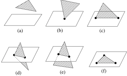
1.9 Alternative deﬁnitions of the contact line for overlapping polygons . . . 20

1.10 Numerical approaches to Coulomb friction (one dimensional case) . . . 23

1.11 Unphysical motion of a block on an inclined slope in numerical simulation ignoring the diﬀerence between static friction and dynamic friction . . . 24

1.12 Artificial data of configuration averages for flow problems with clogging . . 28

1.13 Artiﬁcial data of taking an average over a pressure distribution with a marked dip . . . 28

1.14 Pressure distribution of a single measurement . . . 29

1.15 Improper average of pressure measurements under granular heaps . . . 29

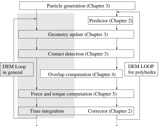
1.16 General DEM ﬂow diagram and the diagram in our DEM implementation for a time integration with a predictor-corrector method . . . 32

2.1 Sketch of the translation and rotation of a rigid body in a space-ﬁxed co-ordinate system and a body-ﬁxed coco-ordinate system . . . 35

2.2 Euler explicit method . . . 40

2.3 Euler implicit method . . . 41

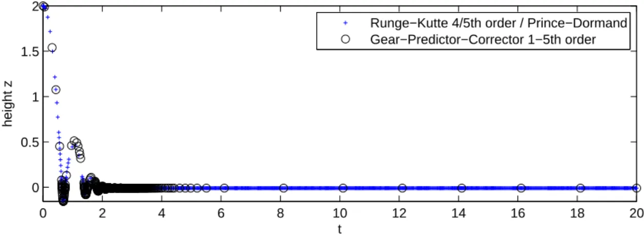
2.4 Simulation of a bouncing ball with the explicit Runge-Kutta method and the Gear-Predictor-Corrector formula . . . 44

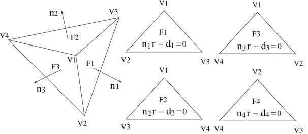
3.1 A sketch of the geometry of a tetrahedron and its topological information of vertices and faces . . . 48

(12)

3.2 An example of the VERT_COORD, FACE_EQUATION, FACE_VERTEX_TABLE and VERTEX_FACE_TABLE array used in the DEM simulation to represent the

tetrahedron in Fig. 3.1 . . . 48

3.3 Various kinds of polyhedra for DEM simulations . . . 49

3.4 Comparison of the polyhedra with 62 vertices and 120 faces generated from Schinner’s and our method . . . 51

3.5 Sketch of a pyramid for decomposing a complex polyhedron. . . 52

3.6 Decomposition of a sub-tetrahedron of a polyhedron . . . 52

3.7 Contact detection via bounding boxes in 2D . . . 56

3.8 Verlet table . . . 57

3.9 Neighborhood table . . . 58

3.10 Sketch of a cell and its neighboring cells needed to be checked in two di-mensions and in three didi-mensions . . . 59

3.11 A case only one particle is larger than the rest in neighborhood table. . . . 59

3.12 Positions of the particles and of the bounding boxes in a one dimensional case for the neighborhood algorithm via sorting . . . 61

3.13 Relative movement of bounding-boxes in one dimension . . . 62

3.14 Embedding of the linear array a for the bounding box positions between a sentinel of extremal values . . . 63

3.15 Relative movement of bounding-boxes in two dimensions . . . 63

3.16 Relative movement of bounding-boxes in three dimensions . . . 64

3.17 Reﬁnement of the contact detection results via bounding circles in 2D . . . 66

3.18 Reﬁnement of the contact detection results via vertex projection in 2D . . . 67

4.1 A point-direction form representation for a triangle . . . 70

4.2 Two intersecting triangles represented by point-direction forms . . . 71

4.3 Possible relative positions of a triangle and a plane . . . 74

4.4 Intersections of two triangles with the two corresponding planes . . . 76

4.5 The sorted intersection segments of two triangles . . . 76

4.6 Overlap of two irregular-shape polyhedra . . . 80

4.7 One intersection point enters twice into the intersection point list . . . 82

4.8 The degenerate cases in the overlap polyhedron computation . . . 83

4.9 The inherited and generated vertices of the overlap polyhedron of two in-tersecting polyhedra . . . 85

4.10 Example of an inherited face and a generated face . . . 86

4.11 Order the vertices on a generated face with respect to the centroid . . . 88

4.12 Order the vertices for a generated face with respect to an edge . . . 89

4.13 Sketches of the contact lines of two intersecting polyhedra . . . 90

4.14 The overlap polyhedron and the contact area and normal . . . 92

4.15 Determination of neighboring features by the overlap bounding box method and the projection method . . . 94

(13)

4.16 Statistics of the eﬃciency of the contact detection algorithm . . . 97

4.17 Fraction of the number of particles which overlap in the contact list . . . . 97

4.18 Statistics of the eﬃciency of the neighboring feature algorithm . . . 98

5.1 The normal direction and tangential direction for two-dimensional particles 100 5.2 Two interacting polyhedral particles and their overlap region . . . 101

5.3 Deformations and overlap in elastic models . . . 102

5.4 Sound propagations in continuum and in discrete systems . . . 103

5.5 Sound wave in the continuum, in a packing of cubes and in a packing of parallelepipeds . . . 103

5.6 Vectors from the center of mass to the contact point for arbitrarily shaped and regular particles . . . 104

5.7 Chains consisting of large-size and small-size particles . . . 104

5.8 Propagation of the maximum velocities in the discrete chain . . . 105

5.9 Sound velocities of the small-particle and the large-particle chain . . . 106

5.10 Two arbitrary-shaped polyhedral particles approaching each other . . . 107

5.11 The time evolution of the volume of the overlap polyhedron . . . 108

5.12 The time evolution of the center of mass of the overlap polyhedron . . . 108

5.13 The time evolution of the contact normal and the elastic force . . . 109

5.14 Sketch of the variation of the total normal force . . . 110

5.15 Deformation of the “tangential spring” in Cundall-Strack friction model . . 112

5.16 Intended behavior for the Cundall-Strack friction model and its actual os-cillatory behavior . . . 113

5.17 Cundall-Strack tangential increment in two dimensions . . . 114

5.18 A simple test for the force models: a cube on an inclined plane . . . 119

5.19 The volume of the overlap region. . . 120

5.20 Normal force and its convergence . . . 120

5.21 Tangential force and its convergence . . . 121

5.22 Position equilibrium of the block on the wedge. . . 121

5.23 Force equilibrium of the block on the wedge. . . 122

6.1 Sketch of a shared memory and a distributed memory computer. . . 127

6.2 Independent loop, forward dependency and backward dependency . . . 127

6.3 Syntax of the loop construct of OpenMP in FORTRAN. . . 130

6.4 Pseudocode of the force computation iterations. . . 133

6.5 Pseudocode of the (inherited) vertex computation iterations. . . 134

6.6 Pseudocode of the (triangular) face intersection computation iterations. . . 134

6.7 Coarse-granular (above) and ﬁne-granular (below) parallelization approach for multi-core machines (in OpenMP style with four cores available). . . 135

6.8 Pseudocode of the parallelized force computation iterations. . . 136

7.1 Sand heap on a mirror . . . 142 vi

(14)

7.2 Granular heap of polygons on top of a zigzag surface . . . 142

7.3 A heap constructed by polyhedral particles on a ﬂat surface . . . 143

7.4 The centers of mass of the particles of the heap. . . 144

7.5 The time evolution of the total energy of the granular heap. . . 145

7.6 The velocity in z direction of a single particle dropped on a ﬂoor. . . 146

7.7 The angular velocity of a single particle dropped on a ﬂoor . . . 146

7.8 Sketches of the dispersion of a laser beam going through a granular system 149 7.9 A laser-sensor pair to measure the strength of the laser beam after dispersion149 7.10 Calibration setup and samples of glass beads used fore experiment . . . 150

7.11 Calibration result: each data point is the average of 80 measurements . . . 151

7.12 Construction and measurement setup . . . 152

7.13 Construction of a quasi-two-dimensional heap and its density measurement 152 7.14 Particles used in the simulation of the quasi-two-dimensional heap . . . 154

7.15 Snapshot of the centers of mass of particles in the quasi-two-dimensional heap154 7.16 Three density homogenization methods for heaps . . . 155

7.17 Moving cell homogenization scheme for density computation . . . 155

7.18 “Proper” and “improper” angles of repose from the experiments . . . 156

7.19 Density results from the experiment with a lifting velocity 1 mm/s . . . 157

7.22 “Practical” and “impractical” angles of repose from the simulations . . . 160

7.23 Density results from the DEM simulation . . . 161

7.24 Pressure “dip” of the heap in the DEM simulation . . . 162

7.25 Construction of a quasi-two-dimensional heap by layered sequence . . . 162

7.26 Density results from the DEM simulation of a layered sequence heap . . . . 163

7.27 No pressure “dip” for the layered sequence heap in the DEM simulation . . 164

(15)

List of Tables

2.1 Gear corrector coefficients for second-order differential equation . . . 43 4.1 Performance comparison of PDTIA (without matrix rank check) and PNTIA 78 4.2 Performance comparison of PDTIA (with matrix rank check) and PNTIA . 79 6.1 Profiling result for the scalar code from a time-based sampling. . . 132 6.2 Profiling result for the parallelized code based function count. . . 137 6.3 Performance for parallel executions on two different multi-core machines. . 139

(16)

Chapter 1

Introduction

In this introduction, we will ﬁrst outline what the systems are for which our DEM-simulation is intended. We then outline those properties of granular materials, which make more conventional simulation approaches problematic, which is why we choose the DEM-method as the approach for simulating granular materials. We then give an overview over other computational methods, to show how they are inadequate to deal with many as-pects which have been outlined in the sections before. We continue with an overview over the alternatives in the force-modeling in DEM-methods, to motivate our choice of polyhe-dra for the shape. Before giving an overview of the thesis, we outline the considerations with respect to the accuracy and stability for DEM-simulations.

1.1 Overview of granular materials

1.1.1 Classiﬁcation

Under granular materials we will understand in the following materials which are made of solid particles which are definitely larger than atoms, and whose deformations under shear are insignificant compared to the dislocation of the center of mass of the particles. The interaction between the surfaces in normal direction of the contact is mostly due to elastic deformation, while in tangential direction, Coulomb friction is significant. The latter leads to static friction, which cannot be neglected, as the usual coefficients of friction are of the order of about half of the normal forces. Very small polymer particles, or the “particles” in gels and colloids, or bubbles in foams, interact by viscous tangential forces and will not be included in our considerations. In other words, it is the quality of the “surface interactions” between the particles which is characteristic for granular materials. A special case would be fracturing, where the particle shape is destroyed, but which nevertheless again leads to granular particles on a smaller scale. The opposite would be sintering, where smaller particles aggregate to larger ones. Both cases will not be treated in this thesis, which

(17)

2 INTRODUCTION

are limited to a purely mechanical treatment of granular materials, due to the amount of thermodynamics surface chemistry involved for a meaningful treatment.

The classical phases or states of matter which are relevant for mechanical considerations are solid (definite shape, definite volume), liquid (definite volume, indefinite shape) and gas (indefinite volume, indefinite shape). The “granular” state is in fact sometimes considered as a “fourth” state, allowing for all the other three: Shape and volume may be definite (granular solid in soil or storage between walls), or volume may be definite, but shape indefinite (usually land- and mudslides, avalanches, liquefaction) or both volume and shape may be indefinite (in granular gases, like dust avalanches, sand-storms and pneumatic transport). The transition between these phases can be induced by mechanical excitations, like vibration and shaking (shaking implies a higher amplitude than vibration), fluid flow (aeolian transport by air, or hydraulic transport by water) or even by electrostatic forces for very fine powders. The focus of this work will be mainly on granular solids and fluids. We discriminate between the macroscopic scale (much larger than the particles size), the mesoscopic or micromechanic scale (of the particle size or fractions of it, depending on the extension of the contact areas), and the microscopic scale (the fine structure of the contacts, with ridges, wear, and the atomic and molecular structure). Our discrete element method treats the granular materials on the mesoscopic scale.

Beyond the macroscopic classification of granular solid, fluid and liquid, another classi-fication are the mesoscopic interactions between the particles. If there are no effects from the surrounding fluids, one speaks of “dry” granular materials if the interaction are only repulsive, or “cohesive” granular materials (usually for particles below 0.5 mm). In this work, we will limit ourselves to dry granular materials, though the force-laws could also be implemented for cohesive materials.

For many processes in granular materials, actually the fluid is relevant, as it inhibits the motion of the granular particles: A typical case is a pile which is driven into some muddy ground or clay, and which starts to move very slowly, when an external force is applied: The granular matrix inhibits the flow of the fluid, as a sponge inhibits flow, while the fluid inhibits the motion of the granular particles by adding cohesiveness. But given enough time, the external force will move the materials nevertheless. The opposite is true for liquefaction during earthquakes, where the fluid destabilizes the granular matrix. These processes cannot be investigated in this thesis, but are mentioned here to show that there are important micro-mechanic aspects beyond dry granular materials. The names of granular materials with fluid depend on the fluid and the mixing ratio. In “suspensions” the particles are only in loose contact in fluids with relatively low viscosity (in air and in water), while in pastes (asphalt, toothpaste) the fluid has high viscosity. The space between the particles is called the “pore space”, while the particles form the “granular matrix”. For porous media, the “granular matrix” can be considered as fixed, only the fluid is in motion, and the volume of the granular phase is usually larger than that of the fluid phase.

(18)

OVERVIEW OF GRANULAR MATERIALS 3

1.1.2 Scales and examples

If we consider granular materials as composed of frictional particles, the smallest grains will be particles for which Coulomb friction is possible. In accordance with the results found in atomic force microscopy, the smallest scale on which Coulomb friction has been found would be of dozens of atoms diameter, i.e. nano-powders. They may be formed from solids, i.e. glassy (no atomic order), crystalline (atomic order) or ceramic (mixture of glassy and crystalline material) particles, where inside the solid the neighborhood between the constituting atoms does not change. Hence, Coulomb friction is possible. While macromolecules may have much higher molecular weight than grains of nano-powders, their molecules are usually partially reorientable and the inter-molecular interactions do not show friction of the Coulomb-type (velocity-independent dynamic friction and static friction), but rather viscous friction. This allows the discrimination between granular materials and polymers based on the type of the interaction and the structure of the constituents. In this work, we focus on a type of particle simulation able to investigate shape effects in a lot of detail. Nevertheless, we concede that shape effects may be irrelevant for some systems of granular materials below the mm-scale, where the cohesive forces will dominate the interaction so that geometric effects become negligible. Nevertheless, even for cement, the size dispersion is relevant for the yield stress, so we think that our approach may also have serious implications for cohesive materials [1].

In principle, rock mechanics would constitute the largest particle scale for granular systems. Nevertheless, with our definition of granular materials as particles which move mostly under the influence of the surface interactions of the constituents, much larger systems can be treated as granular: Shelf ice which floats on water has been treated as a two-dimensional granular material [2] and block-spring-models, simple models with granular interaction are used to model the Gutenberg-Richter distribution of earthquakes, so at least implicitly, continents in some communities are understood as “two-dimensional” granular structure, too.

Granular systems are also found way beyond the earth. Wandering dunes have even be found on Mars. The asteroid belt between Mars and Jupiter has been discussed in the context of granular materials by astrophysicists1[3]. Even if the grain size (maximally several hundred km) would be smaller than that for the continents on earth, at least the extension of the whole system is much larger. Another cosmic aspect of granular matter is the discussion of dark matter and the formation of planets: “interstellar dust” is often mentioned, even if the word “granular material” is usually avoided [4].

1_{e.g. An experiment carried out by European Space Agency: http://eea.spaceflight.esa.int/?pg=} exprec&id=9139&t=2542184240

(19)

4 INTRODUCTION

1.2 Phenomenology and methodology

At least on the terrestrial scale, between nano-powders and rocks, research dedicated to granular materials is found in the fields of (particle size from small to large) powder tech-nology, chemical engineering, process engineering, mechanics, physics, hydrology, civil engineering, geotechnics, geology, rock mechanics and earthquake engineering. As there is no universal governing equation for granular materials, the approach to the modelization varies strongly, depending on the field. In this section, we describe the phenomenology of granular materials and various aspects which have lead to the application of various methodologies. When we discuss the different approaches with respect to the granular phenomenology they are supposed to capture, or fail to capture, some overlap with sec-tions on simulation methods will be unavoidable. Many approaches which have been fruitful in other fields of research (continuum mechanics, molecular dynamics, statistical physics) have been destined to failure with granular materials, at least beyond some nar-row parameter windows. Instead of articles, we will rather cite research groups which are representative for the respective approaches.

1.2.1 Rheology

As long as the rheology of the granular material is of interest, fluid-like models are often employed in powder technology, chemical and process engineering (Nikos Christiakis, at the University of Crete, http://www.tem.uoc.gr/~nchristakis). Rheological approaches work well as long as there is continuous flow due to controlled external excitation, by e.g. fluid flow, vibration or milling. Unfortunately, when the smooth flow breaks down due to clogging, the fluid models neither predict the conditions for the breakdown nor the conditions after the breakdown. Therefore, some researchers in these fields have switched to particle models (Tomas-Group, Univ. of Magdeburg, http://www.uni-magdeburg. de/ivt/mvt/). Similarly, there have been attempts to describe granular materials as very viscous fluids (Jäeger-Group, Univ. of Chicago, http://jfi.uchicago.edu/~jaeger/ group/granular.html). A marked difference to truly viscous fluids is nevertheless that the flow resistance of viscous fluids vanishes with the flow rate, while for granular materials, due to Coulomb friction, the flow resistance is always finite even for vanishing velocity.

1.2.2 Plastic behavior versus elasticity

Classical continuum-approaches via elasticity theory are common in geotechnics. Unfor-tunately, dry granular materials are not “elastic” in the sense that granular assemblies have any resistance against pulling forces. On the contrary, the change of neighborhoods under static friction give nearly optimal plastic behavior, so that some jugglers practice with particle-ﬁlled objects, which don’t roll or jump about when they fall to the ﬂoor. As a workaround for the lack of elasticity, the linear relation for shear, obtained by externally

(20)

PHENOMENOLOGY AND METHODOLOGY 5

Fig. 1.1 Closest packing (left) and reduction of the density (Reynolds dilatancy) after the application of external stresses (right).

Fig. 1.2 Closest packing (left) and shear band formation after application of external stresses (right).

(21)

6 INTRODUCTION

confining the system, are used for the “elastic” parameters. An additional problem is that granular materials may increase their volume under shear, the so-called Reynolds-dilatancy, where the pore-space is increased if the aggregate is sheared while in a closest packing, which means effectively a “negative Young’s modulus”, as the volume increases under the influence of an external force, e.g. Fig. 1.1. In milder form, Reynolds dila-tancy also occurs in shear bands in granular materials, e.g. Fig. 1.2. This as well as the possible plasticity and friction has to be incorporated into the models. Consequently, there is a wide flavor of continuum theories used which are supposed to cure some or all of these problems, including nonlinearities (Dimitrios Kolymbas at Univ. of Innsbruck, http://www.uibk.ac.at/geotechnik/ and Theodoros Triantafyllidis at the University of Karlsruhe, http://www.ibf.uni-karlsruhe.de/). Continuum methods are essentially “mean field” approximations, so no fluctuations in the analytical stress-strain curves are assumed, a stark contrast to the experimental reality and to the results one obtains with particle methods.

1.2.3 Statistical physics

Statistical physics tries to describe macroscopic assemblies by distributions of properties for the constituents. In granular material research, these are often energy dissipation properties (H. Hayakawa, the Univ. of Kyoto, http://www2.yukawa.kyoto-u.ac.jp/ ~hisao/hisao-e.html) or the interaction strength via the dispersion relation (O’Hern, Yale University, http://jamming.research.yale.edu/people.html). In this respect, there is an important diﬀerence between thermodynamics and statistical physics: While thermodynamic results should be independent of the microscopic constituents (the classical heat capacity for gases depends only on the degrees of freedom of a molecule, not on the kind of molecule), statistical physics has to take the character of the microscopic constituents into account (ferromagnetism is limited to very few kinds of atoms, and cannot be deduced for arbitrary materials).

1.2.4 Size- and shape eﬀects

Most researchers who claim to work on statistical physics of granular materials (obtain-ing a macroscopic description depend(obtain-ing on the microscopic structure) are actually try(obtain-ing to obtain thermodynamic descriptions (ignoring the micro-structure) by ignoring size and shape effects. Very often, the attempts are based on spherically symmetric models, though the aggregates of round particles have definitely different properties from non-round par-ticles (angle of repose of only about 20◦ instead of over 30◦, lower strength under triaxial compression etc.). This brings us to the issue of effects of the particle shape on the aggre-gates: while the size has already been mentioned, the role of the shape is equally decisive. The strength of a granular assembly is basically a result of the competition between rolling and sliding of the particles in a granular matrix: For round particles, even large

(22)

coeﬃ-THEORETICAL AND COMPUTATIONAL METHODS 7

cients of friction will not be able to stabilize a granular structure against disintegrating by relative rolling at inter-particle contacts. Ironically, a researcher in the ﬁeld of geotechnics (Matsushima-group, Univ. of Tsukuba) is closest to the attitude of our group by insisting on the importance of the shape. Our conceptual approach is to take into account the micro-mechanics of the granular assembly, the shape and detailed particle contacts. Fur-ther, the full description is by a mechanical theory, where friction turns out as a constraint of motion.

1.3 Theoretical and computational methods

1.3.1 The event-driven method

In general, the event-driven method (ED) or discrete event simulation refers to any sim-ulation method where some process A is simulated, and, when an “event” is detected, another process B is effectuated, and then usually process A is continued [5]. For granular materials, the “event driven” method is a DEM-method based on the collision dynamics of two rigid particles which is obtained from the conservation of momentum. In the “time integration”, the particles fly in (under gravity, parabolic) trajectories, until a collision occurs. At the next time where two particles collide (“event”, therefore event-driven) the simulation for all particles is stopped, the velocities of the colliding particles are dealt with, e.g. for frontal collisions of particles with the same mass the velocity with respect to the collision axis is reversed. For systems of low density, i.e. granular gases, it is very fast for round particles, but as each collision dissipates energy, so that for systems with physical coefficients of restitution, the system becomes too dense to be dealt with via two-particle collisions only. The workaround by many researchers is to “switch off” the coefficient of restitution if a certain density is reached. The larger the system is, the shorter the interval between collisions becomes, so the algorithms become less efficient for larger systems. A (physical) remedy for this problem is not to deal with the whole system as one unit, but partition the system into subsystems, each with a “local clock” [6], so that the time is advanced according to the collisions of neighboring particles, not due to the next collision in the global system. For the event driven method, where the particles are practically “never” in contact, except at delta-like events, the sound velocity depends on the particle density [7]. The event driven method is the simplest example for a rigid-body DEM method, nevertheless, its inability to treat resting or permanent contacts between particles or static configurations makes it useless for most systems with “physical” densities.

1.3.2 Lattice models

Lattice-models for granular materials, as will become clear in the following sub-sections, belong to what at best could be called “semi-quantitative” methods. Nevertheless, as they

(23)

8 INTRODUCTION

have found considerable attention in the ﬁeld, they are outlined here.

Cellular automata

The original meaning of cellular automation in computer science is an algorithm which reacts to each of a finite number of input patterns with a deterministic output. In contrast, in the field of computer simulation in physics, it usually means a simulation method which makes use bits “0” and “1”, so that a bit pattern at discrete time “t” results deterministically in (usually another) bit pattern at time “t+1”. The wide use of cellular automata in physics originates in the field of pattern formation in the 1980s, which came into fashion after the fractals had split of as an independent research interest from the field of chaos and nonlinear dynamics in the 1970s. The scientific fame of Stefen Wolfram, the man behind MATHEMATICA, is basically due to his work on cellular automata. In cellular automata, the bits “0” and “1” are treated as physical entities, in particular, so for granular materials “0” stands for “no particle” and “1” for particle. While the use of the method has no proper physical motivation, it allows very fast simulations with many “particles” (bits). Cellular automata were very popular in the field of “pattern formation” (an offspring of the research on fractals, but with less mathematical rigor), from which many researchers changed to granular materials. As many researchers in the granular community received their basic training in statistical physics of phase transitions, where large system sizes must be computed to reduce finite size effects, the appeal of the method comes from the possibility to simulate “large” systems. Moreover, in statistical physics, critical exponents are determined by the symmetry and the range of the interactions, so that correct exponents could be obtained even when the details of the physics were ignored. Nevertheless, as granular systems are mechanical, not statistical systems, and the correlation length in granular systems is usually limited by the static friction, the potential of cellular automata to allow the simulation of large systems is hardly of any use, compared to the fact that essential part of the physics (Newton’s equation of motion) is lost. Cellular automata have been used for flow problems [8] and the modeling of avalanches in sand piles [9]. The latter article had tailored the avalanching in heap formation according to a power law, similar to the Guttenberg-Richter law for earthquakes, where the frequency is inverse proportional to the magnitude. This triggered a whole new fashion in physics, the quest for “self-organized criticality”, as the inverse power law phenomena were called. Nevertheless, for avalanches in sand heaps, experiments showed significant deviations from the cellular automata predictions [10, 11], so cellular automata are rather more pliable than reliable.

Other lattice models

The basic structure of cellular automata can also be adapted to allow more than only binary outputs [12]. As in the case of cellular automata, the attraction for researchers

(24)

THEORETICAL AND COMPUTATIONAL METHODS 9

lies in the fact that one can determine the outcome of the simulation by ﬁxing unphysical parameters, without being inconvenienced by the basic laws of mechanics.

Tetris

As many researchers are not able to deal with non-spherical particles with proper physical equations of motion, once a lattice algorithm based on the TV-game of “Tetris” was devised to investigate compaction problems (packing densities under external excitations). The fact that it was accepted for the prestigious Phys. Rev. Letter journal demonstrates the need of a simulation of non-spherical particles, rather than the computational prowess of its authors to deal adequately with the problem [13]. While shape is certainly an important parameter in compaction, the friction coefficient and to a lesser degree the filling process are important. Both effects can be only incorporated by accounting for the full equations of motion in the simulation, something which will be always out of the reach of lattice models, which even have to make do with discretized space.

1.3.3 The Monte Carlo method

The Monte Carlo (MC) method is a statistical method based on the use of (usually equally distributed) random (or pseudo random) numbers. Before pseudo random numbers from computers became available, tabulated random numbers were used [14], which were gen-erated by roulette-like machines. Before that, only tabulated outcomes of roulette games in casinos for gamblers were available, e.g. [15], so the name was derived from the most famous of casinos, where the outcomes where regularly posted outside and therefore used for the ﬁrst tables2.

Conventionally one discriminates between “direct” and “importance sampling” Monte Carlo methods. Direct methods are usually used for kinetic problems of trajectories, going back in physics to the mid-60’s for modeling the transport modeling of neutrons [16]. In contrast, importance sampling methods model the underlying stochastic processes, e.g. accept or reject events according to the underlying probability, e.g. the Boltzmann-distribution P = e ( −∆E kbT ) ,

for a change of the energy ∆E, Boltzmann-constant k_b at temperature T, so that changes of the system which increase the energy are exponentially suppressed. If the P is used directly, the method is called a Metropolis-algorithm [17] or M(RT)2 _{algorithm, in allusion} to the initials of the authors of the ﬁrst paper. If instead of P

P′= P 1 + P, 2_{http://www.lehrer-online.de/683293.php}

(25)

10 INTRODUCTION

is used, the algorithm is called “heat-bath algorithm”, which limits the acceptance prob-ability to about 50 % even if P _{≈ 1. This is useful if the acceptance of every Monte Carlo} may lead to a repetition of the initial configurations for certain sampling strategies. In granular materials, hybrids of the direct MC (for the propagation) and the importance sampling (for the interaction) are used [18, 19, 20]. A drawback of the method is its lack of physicality, as the deterministic mechanical behavior must be mimicked by statistical laws. Usually, Newton’s laws cannot be fulfilled, especially the force balance, and stochas-tic collision laws are often also difficult to formulate on a Galilei-invariant basis. Like the lattice-models, the Monte-Carlo method for granular materials belongs to the realm of at best “semi-quantitative” methods. Nevertheless, due to its versatility and success for sys-tems with well-stated thermodynamic properties [21, 22], it has also been tentatively used for granular materials, but without leading to algorithm with actual predictive power.

1.3.4 Continuum dynamics

Some additional remarks, beyond the ones in section 1.2 on continuum mechanics are in order here. Continuum methods are widely and with considerable success used in ma-terial science and fluid dynamics. Nevertheless, for granular mama-terials, they have some significant problems. In this section, we want to discuss some aspects which arise in mod-eling granular materials with structural mechanics methods, rather than fluid dynamics like approaches. While the continuum approximation of metals in structural mechanics can rely on the fact that the discrete constituents are atoms with a size below 10−9 m, in a homogeneous mixture, the grain diameter in granular materials has a much larger variation in size. Another aspect is the mixture: While it is the mission of steel mills to produce metals with a homogenous distribution of atoms, in e.g. geotechnics applications, one cannot necessarily assume homogeneous properties of a soil which must be taken as it is. Accordingly, the experimental input data for the continuum modeling show a much larger variation.

The next conceptual problem is that granular materials, in contrast to metal parts, may not necessarily be stressed below the yield stress, but intentionally beyond: For the outﬂow from a silo, deﬁnitely the shear bands which form at the boundary between moving and non-moving material are relevant. Accordingly, a correct modeling of the transition between “elastic” and “plastic” properties is necessary. The “elastic” properties can be taken into account at least approximately by the linear part of triaxial stress-strain diagrams. Nevertheless, there is no elasticity in the sense of an elastic restoring force, but only a linearity between external stress and reacting strain. While at least this dynamics is similar to a conventional Newtonian mechanics, where the deformation is computed due to the external stresses, for plasticity, the stresses have to be computed based on the external deformation, like in constraint dynamics.

(26)

DEM MODELING 11

rather than having one computing method which adapts itself to the boundary condition. The hypoplastic continuum in geotechnics has already been mentioned, another example is the Savage-Hutter model for avalanches [23].

To conclude, the drawback of continuum dynamics is that the concept itself creates leads to a rather paradoxical approach: In the first step, a continuum approximation for a discrete system must be found, for which impressive names like “homogenization” etc. are used, but finding a smooth description for something what is plagued with jumps is certainly not something which can claim physical or mathematical rigor. In the next step, one is stranded with a partial differential equation for which no exact solution exist, instead one has to deal with well-known artifacts of partial differential equations, e.g. the infinite signal-propagation speed in diffusive terms, where a delta-function-like peak at t = 0 spreads out that for largest distances one can still find a finite amplitude at t > 0. In the next step, because of the lack of an analytical solution, one has to discretize the equation again to solve it on the computer. As long as the problem is one of civil engineering, the problem with the validity is “dealt with” by taking a safety margin of a factor of 2, but that can hardly be considered exact science.

1.4 DEM modeling

Fig. 1.3 Physical situation (a soft sphere is deformed while contacting a plane, left) and the simulation with ﬁnite element method (middle, not penalty method, many degrees of freedom necessary in the discretization) and discrete element method (right, overlapping shapes, only degrees of freedom of the corresponding rigid-body problem necessary).

The discrete element method (DEM, see Fig. 1.3, right) is a method which models inter-particle forces based on elasticity parameters and on the overlap of undeformed particle shapes [24, 25]. The penalty-method for finite element method (FEM) in structural mechanics for contact dynamics simulations uses the overlap between finite element shapes in a similar way [26]. The overlap between particles can be understood as the amount of deformation necessary that the particles could physically occupy the space in their actual configuration. Compared to a finite element method of deformable particles [27],

(27)

12 INTRODUCTION

which need a discretization of the elastic particles, the discrete element method needs only the degrees of freedom which is necessary for rigid bodies: Three in two dimensions and six in three dimensions. For the accuracy, there are hardly any drawbacks, as the only additional information one could gain from the finite element method, internal stresses and strains, are either not of interest, or unreliable due to the fact that the microscopic surface asperities will lead to random alterations of the FEM results anyway. In the flowing we will give an overview of the geometry and force models use in DEM simulations. In the flowing we will give an overview of the geometry and force models used in DEM simulations.

1.4.1 Geometry models

The principle of the DEM-method is to compute the forces proportional to the geometrical overlap of the particles used. The most obvious choice in the first DEM-simulations [24] were disks, so that the overlap problem for two-dimensional particles could in fact be reduced to a one-dimensional intersection problem. Nevertheless, circular or spherical particles mean that the forces involved are basically central forces, while in actual granular materials the particles are not spherical, and the forces are not central forces at all. There are important implications for the force networks of round particles in two dimensions: The force network has basically “weak” and “strong” forces, and the network looks as if made of “meshes” of large forces, so that particle groups interacting with strong forces are embedded in meshes of larger force magnitude. This is an artifact of the round particles, for e.g. ellipses, the mesh-structure vanishes, and the bimodal (strong and weak forces) network becomes a wide, continuous unimodal distribution. Therefore, there is a need of the modeling of non-circular or non-spherical shapes. We will showcase here several aspects of this modelization, the apparent advantages, and the actual drawbacks of different choices of the geometry. As a further aspect, the corresponding two- and three-dimensional models are discussed in the same section. The possibility to generalize the model from two to three dimensions is an important aspect of modeling, as on the one hand, it shows how universal the approach is, on the other hand two-dimensional models allow to gain experience with the simpler lower-dimensional system (stability, time-steps, magnitude of overlap) which are necessary for a successful implementation in three dimensions. Generally, what is necessary for a DEM-computation is the force magnitude, from the overlap, and, for physical torques, a force-direction and a force point, and the latter is also necessary for a physical computation of static friction. Not for all models described below definitions can be found to obtain a smooth variation of force magnitude, force point and force direction when the relative motion of the particle is smooth. This has disastrous effects for the stability of the algorithm. In this section, we discuss the issues related to simulation with soft contacts, where the overlap of the particles are finite: Simulations of rigid contacts, where only point-wise contacts (or point-line or line-face or face-face) contacts can exist are discussed in the section on contact mechanics.

(28)

DEM MODELING 13

Ellipses and their generalizations

A natural next step from round particles to elongated particles would be the choice of ellipses. Nevertheless, it should not be forgotten that the overlap computation should be fast, so that double precision computations should be suﬃcient. A single ellipses can be written in normal form

x2 r2 a + y 2 r_b2 = 1.

with half axes ra and rb. Nevertheless, for two ellipses in arbitrary relative position and

orientation, mixed terms in x, y and xy cannot be eliminated, so to represent two ellipses we need two equations

a1x2+ b1y2+ c1xy + d1x + e1y + f1 = 0, (1.1) a2x2+ b2y2+ c2xy + d2x + e2y + f2 = 0. (1.2) According to classroom geometry, we can obtain the intersection point of the ellipses, which are needed to compute the interaction, by eliminating the y in the above equation, so the intersection points between the ellipses are the solutions of the fourth order equation

Ax4+ Bx3+ Cx2+ Dx + E = 0. (1.3)

Analytically, if all solutions are complex, there are no intersection points in the x−y−plane. Unfortunately, when one implements the approach with double precision floating point numbers, it turns out that it does not work [28]. The computed intersection points are off the actual outlines of the ellipses in the percent-range of the half-axes. The reason can be easily seen when the amount of data in the original representation Eqs. (1.1,1.2) are compared with the equation for the intersection Eq. (1.3): For double precision, the coefficients in Eqs. (1.1,1.2) contain information of 2× 6 × 8 = 96 bytes, compared to 40 bytes for the x_{−coordinates in Eq. (1.3): In the transformations to eliminate y, more than} half of the data have been lost. Actually, this analysis can be confirmed easily by trying out overlap computations of ellipses where the orientation is e.g. parallel to the axes: Because the c₁, d1, e1, c2, d2, e2 drop out of the original equations, the information loss is reduced, and the computations from Eq. (1.3) become more accurate3. Of course, this would not happen in analytical computations, but as long as we are limited to floating point computations for performance reasons, the use of Eq. (1.3) is not feasible. To actually compute the intersection points, Eqs. (1.1,1.2) must be simultaneously solved via Newton iteration. For very elongated ellipses, when one end of one ellipse protrudes over the end of the other, the choice of initial values becomes rather problematic, and the iteration may fail. In principle, the same reasoning applies to “super-ellipses” [29]

_rx_an+y rb

n= 1, (1.4)

(29)

14 INTRODUCTION

with positive n. While the contact line and the force point can be computed easily from the intersection points, in the generalization to three dimensions this is not so easy. First of all, when ellipses are generalized to ellipsoids [30], the intersection lines become spatial fourth order curves, which suffer from the same numerical problem as the intersection points. Further, the definition of a meaningful computation of the overlap volume is also not trivial. The problems are worse for super-quadrics, the generalizations of ellipsoids for three dimensions, so algorithms have been proposed [31], but we have seen no results published with such methods. Problems with the computation of force point and overlap volume are usually circumvented by computing only “penetration depths” instead of the detailed contact geometry (volume, contact line and force point). Nevertheless, as will become apparent in the section on Coulomb friction, the inability to specify a contact point, which also applies to “ellipsoidal potentials” [32] also makes the implementation of static friction impossible. Additionally, as will become apparent later, the inability to assign a contact distance and a contact area in two dimensions or a contact volume in three dimensions makes it impossible to fix the sound velocity of the space-filling packing to the theoretical continuum mechanical value derived from the density and the Young’s modulus. Even if that would be only hypothetical for ellipses and ellipsoids, such packings would be nevertheless possible for n_{→ ∞ in Eq. (1.4), the sound velocity of the continuum} is an important quantity to make sure that the dynamics obeys the basics of elasticity theory.

Clusters of round particles

An alternative of non-spherical particles is the use of clusters of rigidly connected spheres to model granular materials, though molecules have been modeled as rigid assemblies of spheres or spherical potentials before the first particle simulations for granular materials were published. When intersections for e.g. disks can be computed, including overlap, force line and force point, clusters of several discs can be easily modeled as rigidly connected so that the center of mass moves according to the forces on all of these particles, and the orientation changes are computed accordingly. Some researchers [33] who obviously did not grasp the simplicity of this rigid approach connected round particles with springs, which lead to rather wobbly and rather unconvincing particles. For reasonable stiffness, the vibration frequency of the springs would have to be resolved. This approach needs about the same data structures as the rigid connection, only without the average of “heavier” particles and therefore reduced step-size for the time integration. Depending on how realistic the simulations shall be, the clusters can be made up of non-overlapping or of overlapping particles. Some [34] have even gone so far as to produce optimized fitting algorithms for the modeling of given surfaces. While the method of rigidly connected particles is very attractive because it allows to generalize a round particle simulation easily to a simulation of non-round particles, to deal with the artifacts for the friction due to the surface roughness is not so easy. If one puts an elongated particle on a slope, for

(30)

DEM MODELING 15

a given friction coeﬃcient µ, the critical angle θ beyond which a particles will slide not stick is

tan θ = µ.

Nevertheless, if the same coefficient of friction is used for a composite particle with a rough surface, the non-convex surfaces interlock and produce additional tangential forces, so that not even for a two-particle problem (particle sliding on a slope) the correct dynamics will be reproduced. Mixing tangential and normal forces is a severe problem for this kind of simulation: Even for multiple-overlapping particles in the simulations by Matsushima et. al. [35, 36], which was made to reproduce the macroscopic stress-strain curves for different kinds of sand (in Japanese geotechnics, Toyoura-sand is usually the preferred object of investigation), the authors were not satisfied with the results. The Matsushima-group has used very faithful particle modeling in two dimensions, but now uses very rough particle modeling in three dimensions, see Fig. 1.4. Officially, performance reasons are given, but another aspect one could imagine is numerical stability, as turned out by our discussions related to that subject at Tsukuba University in February 2010: Overlapping of many spheres may lead to contacts which are much harder than a single sphere, so that a reduction of the time step becomes necessary. While twice the number of particles would reduce the time step only by a factor of square root of two, it would improve the shape of the particles considerably if overlapping spheres would be used, see Fig. 1.5. Additionally, we have not encountered any detailed discussion on the numerical implementation of the rotational degrees of freedom and the equations of motion in Matsushima’s work, as we have done here in this thesis, so beyond modeling, there may be also additional issues.

Fig. 1.4 Matsushima in 2005 [35] and in 2008 [36]: The two-dimensional simulations are much more faithful to the particle shape than the ones for three dimensions.

Rigidly connected primitives

Apart from spheres and circles, spheres can also be combined with cylinders to reduce the number of primitives and obtain smoother surfaces. In the DEM ﬁeld, cylinders in three dimensions have been combined with spheres to rods [37] and “polyhedra” [38] (or rather skeletons of polyhedra). Nevertheless, as the corners must still be modeled with circles in two dimensions, while surfaces must be modeled with cylinders in three dimensions, the

(31)

16 INTRODUCTION

x

∆

Fig. 1.5 Composite particles made from round particles will have a higher effective Young’s modulus due to the higher number of contacts (larger contact area), as indicated by the 13 dotted lines in the configuration on the right. Three-dimensional configurations would have an even higher number of contacts. This must be taken into account in the choice of the time step: For 13 contacts, and three times the mass of the particle, the time step should be √3/13 ≈ 0.48 or nearly only a half of the corresponding round particle simulation.

problem of interlocking and the wrong allocation of the total granular forces to tangential and normal forces perpetuates. Algorithmically, the inclusion of elongated primitives makes a decision necessary “up to where” the forces of neighboring primitives should be in eﬀect: The connection must be smooth, else for particles with smoothly varying relative position and orientation will vary non-smoothly, and the simulation will become unstable.

Polygons and polyhedra

Polygons and polyhedra are a natural choice for simulating granular particles, as granular particles are “edgy” in the ﬁrst place, and the walls used in technical devices are usually straight (or can at least be modeled by straight lines). Unfortunately, the approach has a bad reputation as being time consuming. For the polygonal code of our group, this is certainly not the case, as in the one used in our research group less than half of the time goes into the overlap computation at least for moderate number of particle corners. Of course, for large number of corners, the update of the particle outline will dominate, but simulations of particles with 128 corners are hardly meaningful, except for control runs to reproduce the results for round particles. The remainder of the computer time goes into the time-integration and the collision detection, which have to be performed also for any other simulation with particles of another shape. Nevertheless, there is an indication that the performance problems of many groups were due to the faulty computation of simulation quantities (e.g. the moment of inertia in the simulations of H.-J. Tillemans4), or careless performance of the overlap computation. In that case, the simulation becomes unstable and usually the users run the simulation with much smaller time step than necessary. While some work has been done at DEM-simulation of polyhedra [39, 40], no simulation

(32)

DEM MODELING 17

results have been published up to now. The conclusion in the granular community is that these codes did not work properly or became unstable easily. Therefore, the subject of this thesis is the generalization of a polygonal simulation to a working and stable polyhedral simulation, while the UIUC group has distributed the work to two theses [41, 42].

Piecewise curves

The use of piecewise curves, like circle segments, shares characteristics of the simulation for ellipsoids, as the contact line intersections are more complicated than for straight lines. There is also a common feature with the composite primitives, as there is a necessity to decide during the overlap computation where the segments end. Arcs of circles have been used [43, 44]. Even (non-convex) shavings of hollow cylinders have been implemented [45]. Surprisingly, splines seem not to be in use in the granular or discrete element community, maybe due to the lack of reliable overlap computations.

Finite element codes

Finite element packages also offer the possibility to model discrete elements from particles made up from finite elements in two [46, 47] and three dimensions [48]. The DEM-functionality is also incorporated into software packages, e.g. in the ANSYS workbench. The interaction between the particles is then computed usually by a penalty method, i.e. the force is proportional to the overlap. The discrete element inter-particle forces can also be interpreted as such a penalty, so the discrete element method could be described as a penalty finite element method without finite elements. Nevertheless, for “usual” stresses far below the yield, the shape of the contacting surfaces is more important for the dynamics than the shape changes from the strains, so the introduction of the deformation only blows up the computational effort by increasing the number of the degrees of freedom.

Another aspect of the finite element methods is that attempts have been made to couple discrete with finite elements [49]. Nevertheless, if the discrete element method is run “fully” dynamically (instead of static or quasi-static calculations), vibrations may be on a timescale close to the particle’s eigenfrequency (which results from the particle mass and the Young’s modulus). The coupling between particles and finite elements is then only possible if the elements neighboring the discrete element particles are of similar size, so that no abrupt changes in the wave resistance (mechanical impedance) R =√Y ρ (Young’s modulus Y , density ρ) occur, else arbitrary reflections of vibrations are possible at the particle-FEM-boundary, and the simulation becomes noisy or unstable. In that case, there is not so much gain from replacing discrete element particles with finite element regions.

(33)

18 INTRODUCTION

1.4.2 Normal force models

In this section, we will give an overview over possible normal force models for DEM simula-tions, and the following explanations will justify our particular choice for the computation the full overlap geometry for our polyhedral DEM simulation.

Penetration depth

d

₁

2 P

₁

2

3 d

P , t=3

P , t=2

P , t=1

Fig. 1.6 Penetration depths of a pair of particles P1 and P2 at three diﬀerent time steps.

The original molecular dynamics code for “soft disks” by Alder and Wainwright [50, 51] used the penetration depth as parameter of the normal interaction strength, and as such is a prototype of a DEM method. This is sufficient to obtain a qualitatively realistic dynamics for round particles, where the forces are basically central forces, so that together with the particle distance, also force point and force direction are determined. While such a minimalist approach is appealing, it should not be forgotten that the minimal computational effort leads also to a minimum amount of information about the contact geometry for more complicated particle geometries. In that case, additional information about the direction of the force, not only the magnitude, is needed. In particular, for simulations of polyhedra, one reason that several projects [52, 53, 54, 55] have not led to the publication of simulation results is in all likelihood that while the absolute value of the penetration depth is a smooth function for smoothly varying relative particle positions, the direction definition is a different matter, and may have led to destabilization of the whole simulation. If one would use the penetration depth, on could define the force direction at those features where (in two dimensions) the contact line is longest and in that direction

DISCRETE ELEMENT METHOD FOR 3D SIMULATIONS OF MECHANICAL SYSTEMS OF NON-SPHERICAL GRANULAR MATERIALS

DISCRETE ELEMENT METHOD FOR 3D

SIMULATIONS OF MECHANICAL

SYSTEMS OF NON-SPHERICAL

GRANULAR MATERIALS

JIAN CHEN

THE UNIVERSITY OF

ELECTRO-COMMUNICATIONS

GRADUATE SCHOOL OF

ELECTRO-COMMUNICATIONS

A DISSERTATION SUBMITTED FOR DOCTOR

OF PHILOSOPHY IN ENGINEERING

DISCRETE ELEMENT METHOD FOR 3D

SIMULATIONS OF MECHANICAL

SYSTEMS OF NON-SPHERICAL

GRANULAR MATERIALS

APPROVED BY SUPERVISORY COMMITTEE:

CHAIRPERSON: ASSOC. PROF. Hans-Georg Matuttis

MEMBER: PROF. Hiroshi Maekawa

MEMBER: PROF. Takeshi Miyazaki

MEMBER: PROF. Takashi Kida

MEMBER: PROF. Tomio Okawa

Copyright

by

JIAN CHEN

2012

非球形粒子を用いた粉粒体力学三次元シミュレーションの

ための離散要素法

陳 健

概要

Discrete Element Method for 3D Simulations of

Mechanical Systems of Non-Spherical Granular

Materials

Jian Chen

ABSTRACT

Contents

List of Figures

List of Tables

Chapter 1

Introduction

1.1

Overview of granular materials

1.2 Phenomenology and methodology

1.3

Theoretical and computational methods

1.4

DEM modeling

x

∆

d

d

1

2

P

1

2

2

2

3

d

P , t=3

P , t=2

P , t=1

陳健

₁

₁