Graduate School of Science
Department of Physics
Diversities out of the observed proto-planetary
disks: migration due to planet-disk interaction
and architecture of multi-planetary systems
(®
®
®ß
ß
ß
L
L
L
⇧
⇧
⇧8
8
8à
à
à
¿
¿
¿ú
ú
ú⌃
⌃
⌃↵
↵
↵I
I
I.
.
.∫
∫
∫“
“
“Ï
Ï
Ï⌥
⌥
⌥à
à
à
—ú
ú
ú⌃
⌃
⌃á
á
á.
.
.˘
˘
˘÷
÷
÷+
+
+H
H
HK
K
K;
;
;#
#
#(
(
(∫
∫
∫Í
Í
Íà
à
à
¿
¿
¿.
.
.j
j
jü
ü
ü)
Shijie Wang
A thesis submitted to
the graduate school of science,
the University of Tokyo
in partial fulfillment of
the requirements for the degree
of
Master of Science in Physics
As more and more exoplanets have been discovered at a staggering rate, we gradually realised that the population of the exoplanets exhibits a great diversity. We have seen not only the wide-range distribution of the planetary architectures over various parameter spaces, but also specific phenomena that intrigue theorists for a long time, such as Hot Jupiters, large spin-orbit misalignment and free-floating planets. While many models have been proposed to account for these observational facts and some of them can yield very promising results, these theories have not yet been examined in the realistic situation, as their investigations start from either fine-tuned or purely theoretical initial conditions.
In 2015, Atacama Large Millimeter Array changed this picture by releasing the high-resolution image of the HL Tau protoplanetary disk. This image revealed the concentric rings and gaps on the HL Tau disk, which are commonly interpreted as the results of planet formation. Following this assumption, we can extract the configuration of HL Tau system and use that as the initial conditions for planetary evolution to see whether the diverse configurations of the observed planetary systems can be reproduced.
The main objective of this thesis is to investigate the evolution outcomes of the HL Tau system based on initial conditions deduced from the current observation. We first reviewed the basic structure of the protoplanetary disk, the planet-disk interaction, and the observational facts about the HL Tau. We then presented our theoretical methodology and numerical approaches to evolve the HL Tau system. We considered the combined e↵ects of the planetary migration and accretion by adopting the exiting migration theory and modelling the disk structure that hosts multiple planets. We also implemented the migration and accretion model to the N -body numerical simulation framework which was subsequently used for simulations. In total we examined 75 cases of 3-planet system, and each system was evolved for up to 0.1 Gyr after disk dispersal.
We present the results at two di↵erent epochs, one at three times the disk lifetime(3⌧disk) and
one at 0.1 Gyr after the disk dispersal. For each epoch, we present the example evolution and explain the pattern that emerged from the plots. We also break down the results in parameter spaces of flaring index, disk lifetime and viscosity. Our main findings include:
1. After 3⌧disk, the final semi-major axis of planets ranges from 0.007 au to 30 au, while the
planet mass ranges from 0.4 MJ to 10 MJ, which is significantly more diverse than the
previous study on HL Tau.
2. When the flaring index, disk lifetime and viscosity increase, the final semi-major axis decreases and the final mass increases, and vice versa.
3. All planet systems remain stable up to the simulation time. No instability has been observed.
We also find that all systems survive much longer than the lower limit of instability time pre-dicted from the mutual hill radius, and from which we conclude that the disk-planet interaction at early stage of the planetary evolution can stabilise the system. We further study the sta-bility by investigating the period ratios and the separation between adjacent planets in their mutual hill radius. We find that the migration coupling prevents the planet-pair from entering resonance states smaller than 2 : 1 resonance.
I would like to express my sincere gratitude to my supervisor, Prof. Yasushi Suto, for his continuous guidance and support during the whole course of my Master programme. From his teaching, I have learned not only the knowledge and techniques that are indispensable for physics research, but also the correct altitude and responsibility that a physics researcher should have, which are invaluable to my future study. Next I would like to thank my principal collaborator, Dr. Kazuhiro Kanagawa, who briefed me on this project with patience and explained many aspects of the protoplanetary disk research with great details. I would also like to thank another collaborator, Toshinori Hayashi, who did the preliminary work with me, contributed to many fruitful discussions and continued encouraging me during the project. I would like to thank my defence committee members, Prof. Fujihiro Hamba and Prof. Kipp Cannon. Their precious comments are greatly appreciated and play an important role in the later revision of this thesis. I also want to thank other members of UTAP/RESCEU who contributed to the discussions of this project.
Finally I would like to thank my parents who provides me both care and financial support, which I will remember and appreciate for my entire life.
Abstract i
Acknowledgements iii
1 Introduction: an Overview 1
2 The Protoplanetary Disk 4
2.1 Structure . . . 4 2.1.1 Vertical structure . . . 4 2.1.2 Radial Structure . . . 6 2.1.3 Temperature Profile . . . 8 2.2 Evolution . . . 10 2.2.1 Classical Picture . . . 11
2.2.2 Solutions of the surface density ⌃g . . . 12
2.2.3 Viscosity and the Shakura-Sunyeav ↵ prescription . . . 13
2.2.4 Stability of the disk . . . 14
2.2.5 Disk Dispersal . . . 15
3 Planetary Migration 18 3.1 The Resonant Torques . . . 18
3.2 Type I migration . . . 20
3.3 Type II migration . . . 21 v
vi CONTENTS
4 The HL Tau system 23
4.1 Disk Structure and Properties . . . 23
4.2 Planetary signatures: the gap structure . . . 24
4.3 Previous Study: Planetary Dynamics in HL Tau System . . . 26
5 Methods 28 5.1 Theoretical framework . . . 28
5.1.1 Equations of Motion . . . 28
5.1.2 Model of the Disk Structure Hosting Multiple Planets . . . 30
5.1.3 Accretion Model . . . 31
5.1.4 Migration Model . . . 32
5.2 Numerical Approaches . . . 33
5.2.1 Simulation Environment . . . 33
5.2.2 Parameters and Initial Conditions . . . 35
5.2.3 Simulation Structure . . . 35
6 Results 37 6.1 Evolution during the Disk-planet Interaction (t < 3⌧disk) . . . 37
6.1.1 A Typical Example of Planetary Evolution . . . 37
6.1.2 Distribution of Planet Mass and Semi-major axis . . . 41
6.1.3 Parameter Dependence of Planetary Mass and Semi-major Axis . . . 41
6.2 Stable Evolution for the First 0.1 Gyr after the Disk-dispersal . . . 43
6.2.1 Comparison with the Previous Criteria in terms of the Hill Radius . . . . 44
6.2.2 Hints to the Stability: the Period Ratios . . . 46
7 Conclusion 50 7.1 Summary . . . 50
A.1 The Energy Conservation Test . . . 52 A.2 Reproduction of result in Simbulan et al. (2017) . . . 53
Bibliography 54
4.1 Ring properties and gap properties of HL Tau . . . 25 4.2 HL Tau initial conditions used by Simbulan et al. (2017). . . 26
5.1 Input parameters and variables . . . 34
A.1 Comparison between Simbulan et al.’s result and the reproduction test result . . 53
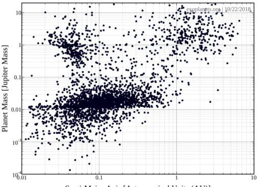
1.1 Mass against semi-major axis of exoplanets. Exoplanets.org (2018) . . . 2
2.1 Illustration of the basic set-up. . . 5
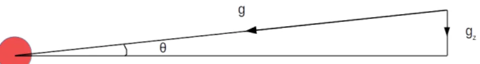
2.2 Illustration of the flux from the star. . . 8
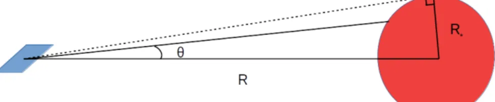
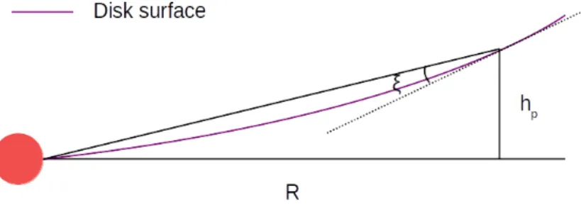
2.3 Illustration of a flared disk. . . 9
2.4 Illustration of the magnetorotational instability(MRI) . . . 15
2.5 Illustration of the thermal winds launched due to photoevaporation. . . 16
3.1 A gap(black color) carved by a giant planet(light dot in the gap) in a hydrody-namical simulation . . . 21
4.1 The HL Tau image . . . 24
4.2 An example semi-major axis evolution of a 5-planet system from the initial con-ditions specified by Simbulan et al. (2017). . . 26
5.1 Accretion rate against planet mass . . . 31
5.2 The Migration timescale . . . 32
5.3 Comparison between the initial locations of the planets in Simbulan et al. (2017) and our simulation. . . 35
5.4 Illustration of the timeline of the two-stage simulation . . . 36
6.1 An example of the evolution of a, m, e and ⌧a for planets 1, 2 and 3 (f = 0.25, ⌧disk = 2 Myr and ↵ = 3⇥ 10 4). . . 38
6.2 Global evolution of the gas surface density profile and the evolution of gas surface density at each planet’s location. . . 39
6.3 2-D visualisation of the disk gas surface density at di↵erent epochs. . . 40
6.4 Overall Distribution of Planets after disk phase . . . 41 xi
6.5 Semi-major axis and Mass dependence on flaring index. . . 42
6.6 Semi-major axis and Mass dependence on disk lifetime ⌧disk. . . 42
6.7 Semi-major axis and Mass dependence on viscosity ↵. . . 42
6.8 Evolution of the semi-major axis and eccentricity for three planets (f = 0.25, ⌧disk = 2 Myr and ↵ = 3⇥ 10 4). . . 44
6.9 Plot of Kmin and Kavg against the semi-major axis/au of the innermost planet after 3⌧disk. . . 45
6.10 Histograms of the period ratios. . . 47
6.11 Contour Map of the Period Ratio . . . 48
6.12 Evolution of the period ratios with di↵erent f, ⌧disk, ↵. . . 49
A.1 Result of the energy conservation test. . . 52
A.2 Final distributions of the remaining planets . . . 54
Introduction: an Overview
Human beings have a long history of observing planets, which can be traced back to Babylonian period when Mercury, Venus, Mars, Jupiter and Saturn were, for the first time, identified by the ancient astronomers(Sachs, 1974). However, only after the telescope was invented and Newton’s law of universal gravitation was formulated, were astronomers able to discover more planets inside the solar system as well as to acquire more details about those planets that had already been identified. The 7th planet Uranus was discovered in 1781 by William Herschel using his own telescope, and then Neptune by Galle in 1846 inspired by the calculation from the French mathematician Le Verrier, marking the culmination of the 19th century’s celestial mechanics. As the observation techniques continue to evolve over the years, nowadays we have a repertoire of means to unveil the remaining unknowns of our solar system. For example, in 1970s we sent the Voyagers space probes which visited Jupiter, Saturn and Uranus in succession and then sent back unprecedented in-situ observation data. As similar projects are going to be launched in a steady pace, our solar system will eventually be thoroughly studied in the foreseeable future.
In contrast to the good knowledge that we have on our solar system, our understanding of the exoplanetary systems is just at the very beginning. Though historically many attempts had been made, it was generally believed that there was no confirmed observation until the year of 1992, when the first exoplanet was discovered to be orbiting around the pulsar PSR 1257+12 by analysing the pulsar timing variations(Wolszczan & Frail, 1992). Observing exoplanets via direct imaging is challenging because exoplanets are both tiny compared to the star(⇠ 10 3 in
mass ratio) and generally distant from the earth, which are light years away compared to a few AUs for planets in our solar system. Therefore, other supplementary methodologies, such as transit photometry, Doppler spectroscopy(radial velocity) and gravitational micro-lensing, were developed for the sake of more efficient observation. Since the beginning of the 21st century, particularly after the launch of the Kepler space observatory, the number of newly discovered exoplanets per year grows rapidly. Up to now, in total 5,311 exoplanets have been identified, including both confirmed planets and Kepler candidates(Exoplanets.org, 2018).
While the fast-growing number of the exoplanets that had been discovered brought us into a new world never seen before, new intriguing problems also appeared along side with the discoveries. A good example is the Hot Jupiter(HJ), which is a Jupiter-size planet however very close to its hosting star. In 1995, for the first time, a planet orbiting a main-sequence star was detected, namely the 51 Pegasi b. This planet, later considered as a HJ, has a minimum
2 Chapter 1. Introduction: an Overview
mass(m sin i) 0.46MJ and an orbital period only 4.23 days(Mayor & Queloz, 1995). Later many
other HJs were discovered via the radial velocity method, indicating that HJs were not rare in our galaxy. Contrary to the previous understanding of the Jupiter-size planets, the existence of HJ nevertheless challenges the traditional in-situ formation theory of planet, as a contradictorily much larger orbit is necessary to have the sufficient mass-accretion for such a massive planet to form. We may also realise that the formation of HJ is not the only problem that ba✏es those exoplanet scientists: many related others, such as the large spin-orbit misalignment and number estimate of free floating planets, all remain as open questions. It thus poses a need to find the physical explanations to cater these new discoveries.
Figure 1.1: Mass against semi-major axis of exoplanets. Exoplanets.org (2018)
Throughout the years, many new insights have been added to the old theoretical framework, which greatly enriched our understanding of the exoplanetary evolution. To reconcile HJ’s mass to its position, theorists came out with the Type II disk migration model (e.g., Lin et al., 1996) and later-proposed dynamical evolution model(e.g., Wu & Murray, 2003; Nagasawa et al., 2008). The spin-orbit misalignment may be either due to the famous Kozai mechanism(Kozai, 1962) or the primordial misalignment interpretation due to the binary evolution(Batygin, 2012). While these new theories can partially solve the contradictions, their initial conditions are either fine-tuned to specific purposes or purely theoretical. A new challenge is: “can we find the realistic initial conditions to test the validity of these models?”
Important clues have been brought from the ground-breaking observation of Atacama Large Mil-limeter Array(ALMA) on the protoplanetary disks. In 2015, the high resolution image(Partnership et al., 2015) on the HL Tau system taken by ALMA revealed the concentric ring and gap struc-ture on the disk, which were commonly interpreted as a result of the gap-opening process due to the formation of planets. If this interpretation is correct, it is possible that we can then extract the initial conditions of the planetary system from the properties of the gaps. Even some pa-rameters like orbital phases cannot be directly inferred from the observation, this discovery can still serve as a strong constraint on the initial conditions. Simbulan et al. (2017) took this idea by connecting the observation on HL Tau disk to the initial planetary configurations and then
evolved the system to Giga-year time-scale. With a particular focus on creating the unstable configurations, their research showed that given the range of parameters that they surveyed, the HL Tau system can produce HJ candidates and planet ejections, as well as diversely-distributed planetary systems.
The pioneering work from Simbulan et al. (2017) is inspiring, and it can be extended further by considering the e↵ects of the planet-disk interactions. Since HL Tau is only one-million-year old and the disk usually has a lifetime of a few million years, we may expect that the migration and accretion will take place for the rest of the disk lifetime, which can further shape the configurations of the planetary system just after the disk dispersal. It is not well understood that whether the combination of migration and accretion will impact on the evolution outcomes of the planetary system, such as the diversity and stability. Based on this motivation, we start this research to investigate on the future of planets emerged from HL Tau in a more realistic physical picture.
This research aims to see if the diverse configurations of the exoplanetary systems can be repro-duced using initial conditions derepro-duced from the observed protoplanetary disks, particularly the HL Tau disk. our approach consists of mainly two parts, the disk modelling and simulation. In the disk modelling, we consider the detailed migration and accretion processes of planets inside the disk and also the feedback to the global disk density profile due to individual planet’s accre-tion. In the numerical simulation, we incorporate and implement the planet-disk interactions into the simulation environment and subsequently use the enhanced N -body numerical code to evolve the systems. We analysed the results by showing the patterns emerged, interpreting the physical origins and comparing with the results from other past research. Finally we conclude that to what extent that we can reproduce a diverse population of planetary systems within the range of initial conditions that we survey during the project and what are the impacts of the planet-disk interaction on the final configurations of planetary systems.
We begin by reviewing the protoplanetary disk, the planet-disk interactions and the HL Tau system in Chapter 2, 3, and 4, respectively. In Chapter 5 we explain the methodologies of this research, including both disk modelling and numerical approach. In Chapter 6 we present our discoveries from the numerical simulations and in Chapter 7 we summarise our research and discuss the future work.
Chapter 2
The Protoplanetary Disk
The protoplanetary disk(PPD) is the disk-structured objects that have been observed to be around young stars with a lifetime of a few million years. Commonly recognised as the birthplace for planets, PPD is mainly composed of dust and gas, which structure can be well described by the model based on quasi-equilibrium state. The structure of the PPD strongly shapes the migration and accretion of the planets that form inside the disk; in addition, since the evolution of PPD tightly couples with its structure as well, both the structure and evolution of the disk deserve equal attention while the overall influence on the evolution path of the planet is considered. The review below generally follows the book Armitage (2010) and the review paper Armitage (2015).
2.1
Structure
While considering the structure of the disk, we adopt the approximation that the disk evolves axisymmetrically and slowly enough that the quasi-equilibrium state can be applied at any instant. Starting from the assumptions, we will mainly consider the vertical structure, radial structure and temperature profile of the disk. We use the cylindrical coordinate system (R, z) centered at the star and align the z-direction with the total angular momentum. We define T (R, z), ⌦(R, z) and v = (vR, v , vz) to be the temperature, angular velocity and velocity of
the gas, and use the subscript ‘dust’ to distinguish the respective quantities that associate with the dust from those that associate with the gas. We also define ⇢(R, z) and ⌃(R) to be the density and surface density. Particularly, the density and surface density of the gas are denoted as ⇢g and ⌃g to avoid any confusion.
2.1.1
Vertical structure
The vertical structure of the PPD can be derived by considering the hydrostatic equilibrium, that is, the balance between the gravitational force exerted by the star and the gas pressure. In order to proceed, three further assumptions have to be introduced:
(i) the disk is vertically isothermal,
(ii) the disk is not self-gravitational, i.e., the disk mass to the stellar mass ratio is much smaller than unity, and
(iii) the disk is geometrically thin.
If we assume irradiation from the star is the only source to heat up the disk, the temperature of the disk is only a function of the cylindrical distance to the star, and thus the first assumption is reasonable. The second assumption ensures that the star is the only source of the gravity which shapes the disk. Finally, the third assumption ensures that the hydrostatic equilibrium is valid as generally pressure inside a disk is small due to the large surface to volume ratio of the disk that favors e↵ective cooling. Therefore, geometrically-thick disks cannot balance the gravity by the gas pressure and only thin disks are relevant to the later discussion.
Figure 2.1: Illustration of the basic set-up.
From hydrostatic equilibrium, we can write down the following equation: 1 ⇢g dP dz = GM⇤ R2+ z2 sin ✓, dP dz = GM⇤ R2+ z2 z (R2+ z2)1/2, ⇢g = GM⇤z (R2+ z2)3/2⇢g, (2.1)
whereG is the gravitational constant, P is the gas pressure, and M⇤ is the mass of the star. From the isothermal equation of state, we have P = ⇢gc2s, where cs is the sound speed. Substituting
to equation (2.1), one obtains
c2sd⇢g dz =
GM⇤z
(R2+ z2)3/2⇢g. (2.2)
(2.3) Equation (2.2) can be integrated to give
⇢g = ⇢g,0exp GM⇤ c2 s(R2+ z2)1/2 . (2.4)
Consider the case when z ⌧ R. Given the Keplerian orbital velocity at the mid-plane ⌦K ⌘
p
GM⇤/R3, We define h as the scale height that takes the form
h⌘ cs ⌦K
6 Chapter 2. The Protoplanetary Disk
Equation 2.4 can then be re-expressed as
⇢g = ⇢g,0exp z2/2h2 , (2.6)
and ⇢g,0is the gas density at the mid-plane. Further we can write the mid-planet surface density
as ⌃g =
R 1
+1 ⇢dz and obtain the following relation for ⇢g,0 and ⌃g:
⇢g,0 = 1 p 2⇡ ⌃g h . (2.7)
Equation (2.6) shows that the vertical density profile follows the Gaussian distribution. At a range where z/h is around unity, even the full treatment which does not assume condition z ⌧ R produces a density ⇢g that only deviates slightly from the Gaussian profile. Although
there exist other factors which can cause significant deviation from the Gaussian profile, such as the non-isothermal temperature profile, magnetic pressure(e.g Hirose & Turner (2011)), etc., the detailed discussion of these e↵ects is beyond the scope of this review.
2.1.2
Radial Structure
Compared to the relatively trivial derivation of the vertical density profile, the radial density profile of the disk involves detailed considerations of the transport of the angular momentum and therefore will be discussed later in Section 2.2. Nevertheless, when the surface density ⌃g and temperature T distribution are known, the orbital velocity of the gas v ,gas at the
mid-planet can be derived from the Euler equation by considering force balance in the radial direction @v @t + (v· r)v = 1 ⇢grP r , (2.8) where is the gravitational potential. Since we are interested in the steady state of the disk, @/@t⌘ 0. Taking only the radial component of equation (2.8), we have
v2 R = GM⇤ R2 + 1 ⇢g dP dR. (2.9)
Assuming ⌃g / R and T / R and using the relations:
c2s / T, (2.10) ⇢g / ⌃g h , (2.11) we get P / R 32 / Rn, (2.12)
where we define n⌘ 32 . Substitute the expression of P into equation 2.9 and define the mid-planet Keplerian speed as vK ⌘ ⌦KR ⌘
p
GM⇤/R, the final result is
v2 R = v2 K R + c2 s P dP dR, (2.13)
Hence, we can obtain v as v = vK 1 + nc 2 s v2 K 1/2 , = vK " 1 + n ✓ h R ◆2#1/2 . (2.14)
It can be concluded here that the di↵erence between the gas speed v and Keplerian speed vK is in the order of square of h/R. Although this deviation is only a tiny fraction of the
Keplerian speed(for example, when n = 3 and [h/R]R=1 au = 0.05, the fractional di↵erence (vK v )/vK is 0.4 %), this di↵erence is vitally important in considering the growth of particles
inside the disk: since large particles orbit at Keplerian speed, they will experience a headwind while moving inside the sub-Keplerian disk, therefore losing angular momentum due to the viscous drag and moving inwards in a spiral.
The above derivation only considers the Keplerian speed deviation at the mid-plane. More detailed treatment, provided by Takeuchi & Lin (2002), also includes the vertical dependence. Using the same set-up, their result gives
⌦⇡ ⌦K " 1 + 1 4 ✓ h R ◆2✓ + 2 3 + z 2 h2 ◆# , (2.15)
Considering the o↵-plane Keplerian orbital velocity ⌦K,z written as a function of z:
⌦K,z = GM⇤ (R2 + z2)3/2 1/2 , = ✓ GM⇤ R3 ◆1/2 1 +⇣ z R ⌘2 3/4 , ⇡ ⌦K 1 3 4 ⇣ z R ⌘2 . (2.16)
Therefore, to the first order to (z/R)2, we obtain
⌦ ⌦K,z ⇡ 1 4 ✓ h R ◆2 ⌦K + 2 3 + ( + 3)⇣ z h ⌘2 . (2.17)
Choosing typical values as = 0.5 and = 1, when ⌦ ⌦K,z = 0, we have
z h ⌦=⌦K
⇠ 1.48.
The result shows that near the mid-plane region below z ⇠ 1.48h, particles rotate faster than the gas and therefore experience a headwind; otherwise, particles rotate slower than the gas.
8 Chapter 2. The Protoplanetary Disk
Figure 2.2: Illustration of the flux from the star.
2.1.3
Temperature Profile
To investigate the temperature profile of the PPD, one may assume that the PPD is in thermal equilibrium, and what remains is to find the temperature at which the energy gain and loss balance out each other. There are mainly two sources that the PPD can gain thermal energy from: the irradiation from its hosting star and the gravitational energy released by the accretion matter. On the other hand, the PPD also loses energy through re-emission process. In the following derivation we will start from a simplified disk model, which is the razor-thin and passive disk. If the disk energy income can be solely determined by the irradiation from the hosting star, the disk is called ”passive” and thus the temperature profile will be determined by its geometrical shape. A razor-thin disk will then ensure that the mid-plane of the disk intercept all the radiation and then re-emit in black body spectrum.
Consider a star in radius R⇤ with a constant stellar surface brightness I⇤. Let ✓ and be the polar and azimuthal angles. If we write the unit vector ˆn of the light direction as (sin ✓ cos , sin ✓ sin , cos ✓), then the light flux F can be expressed as
F = Z I⇤(ˆn· ˆx)d⌦ = Z I⇤sin2✓ cos d✓d . (2.18)
Since only half of the star can contribute to the total flux, equation (2.18) is integrated over 0 < ✓ < sin 1 R⇤
R and ⇡/2 < < ⇡/2 and we obtain
F = I⇤ Z ⇡/2 ⇡/2 cos d Z sin 1(R ⇤/R) 0 sin2✓d✓ = 2I⇤ 1 2 1 4sin 2✓ sin 1(R ⇤/R) 0 = I⇤ 2 4sin 1 ✓ R⇤ R ◆ R⇤ R s 1 ✓ R⇤ R ◆23 5 . (2.19)
The brightness of the star at its surface can be related to the e↵ective temperature of the starby using the Stefan-Boltzmann law (Rybicki & Lightman, 1979)
I⇤ = F ⇡ =
T4 ⇤
⇡ . (2.20)
For one side of the disk, the flux F = T4. Substituting back to both sides of the equation
(2.19) gives ✓ T T⇤ ◆4 = 1 ⇡ 2 4sin 1 ✓ R⇤ R ◆ R⇤ R s 1 ✓ R⇤ R ◆23 5 . (2.21)
In the region far from the star, i.e., R⇤ ⌧ R, equation (2.21) is reduced to a simple power law temperature profile
T / R 3/4. (2.22)
Using the relation c2
s / T and h ⌘ cs/⌦K, the aspect ratio is
h R / R
3
4·12+32 1 / R1/8. (2.23)
Defining the flaring index f through (h/R) / Rf, the temperature profile for a razor-thin,
passive disk gives f = 0.125. This shows that when R increases, the aspect ratio also increases, resulting in a disk which is called ‘flared’.
Flared disk
We note that the above result is over-simplified in many aspects. At large R, the flared part of the disk contributes to additional absorption area and therefore gaining higher temperature than the originally-assumed razor-thin disk. The full solution that takes account of the flaring e↵ect can be derived in a similar way, but a simplified consideration that takes the limit R⇤ ⌧ R and the star to be a point source is sufficient to understand the e↵ect qualitatively.
Figure 2.3: Illustration of a flared disk.
Following the arguments in Armitage (2010), we define a maximum absorption height hp at
radius R and then define ⇠ as the angle between the incoming radiation and the tangent of the local disk surface:
⇠ ⌘ dhp dR
hp
R. (2.24)
10 Chapter 2. The Protoplanetary Disk
we can equate the local heating rate(left-side) and the cooling rate(right-side) as ⇠ ✓ L⇤ 4⇡R2 ◆ = T4. (2.25) Using L⇤ = 4⇡R2⇤ T⇤4, we obtain ✓ T T⇤ ◆4 = ⇠ ✓ R⇤ R ◆2 , (2.26) T / ⇠1/4R 1/2. (2.27)
This shows that at large radii the temperature of a flared disk drops slower than that of a razor-thin disk, as R increases(c.f. equation (2.23)).
So far we also only consider a single-composition model of the disk, where in reality the dust dominates the absorption inside the disk and thus its radiative thermal properties have to be taken care of. We define the ✏ as the efficiency of emission/absorption of dust relative to the black-body. When the wavelength of the incoming radiation is smaller than the radius of the dust, the dust absorbs and emits like a blackbody with emissivity ✏ = 1; when the wavelength is longer than the dust radius, the dust emissivity drops with ✏/ 1. Using the same thermal
equilibrium argument, the dust temperature Tdust can be expressed as
Tdust T⇤ = ✓ ✏⇤ ✏dust ◆1/4✓ R⇤ 2R ◆1/2 = ✓ Tdust T⇤ ◆1/4✓ R⇤ 2R ◆1/2 , ) Tdust T⇤ = ✓ R⇤ 2R ◆2/5 / R 2/5, (2.28)
where ✏dust is the weighted emissivity of the dust averaged over the dust thermal emission, and
✏⇤ is the weighted emissivity for the absorption averaged over the stellar spectrum. The above analysis follows the two-layer model developed by Chiang & Goldreich (1997). For a star with 0.5 M mass, 2.5 R radius and 4000 K e↵ective temperature, the dust temperature profile is
Tdust = 550 ✓ R 1 au ◆ 2/5 K. (2.29)
2.2
Evolution
The PPD evolves as the gas keeps accreting onto the central star, whereas the disk wind launched by the magnetic field and photoevaporation e↵ect continues to cause the mass loss. The movement of the gas is governed by the gain and loss of the angular momentum. Therefore, the key idea to understand the evolution of the PPD is to understand how the angular momen-tum is transferred and redistributed within the disk. Starting from the basic conservation laws, we can write the hydrodynamical equations in the context of the PPD and then obtain various characteristics of the disk evolution. The following review mainly follows Pringle (1981).
2.2.1
Classical Picture
The classical picture of the disk evolution concerns the evolution of a vicious, axisymmetric and geometrically-thin disk. Construct the cylindrical coordinate system (R, z) as before, the conservation of mass and angular momentum can be written as
R@⌃g @t + @ @R(R⌃gvR) = 0 (2.30) R@ @t(R 2⌦⌃ g)+ @ @R(R 2⌦· R⌃ gvR) = 1 2⇡ @G @R. (2.31)
Compared with equation (2.8), equation (2.31) is derived from the Navier-Stokes equation which also takes account of the viscosity. G on the right side of the equation (2.31) is the vicious torque that acting on the edge of the annulus:
G = 2⇡R· ⌫⌃gR
d⌦
dR · R, (2.32)
where ⌫ is the kinematic viscosity. From equation (2.30) we have @⌃g @t = 1 R @ @R(R⌃gvR). (2.33)
Substituting equations (2.33) and (2.32) to equation (2.31) and use prime to denote dRd , then
R2⌦ @ @R(R⌃gvR) + R⌃g @ @t(R 2⌦) + @ @R(R 2⌦· R⌃ gvR) = @G @R, (2.34) R⌃g @ @t(R 2⌦) + R⌃ gvR @ @R(R 2⌦) = @ @R(v⌃gR 3⌦0). (2.35) Since dtd ⌘ @ @t + vR @ @R, R⌃g dR dt (R 2⌦)0 = @ @R(v⌃gR 3⌦0), (2.36) R⌃gvR= 1 (R2⌦)0 @ @R(v⌃gR 3⌦0). (2.37)
Substituting equation (2.37) back to equation (2.33), @⌃g @t = 1 R @ @R 1 (R2⌦)0 @ @R(v⌃gR 3⌦0) . (2.38) Using Keplerian ⌦/ R 3/2, @⌃g @t = 3 R @ @R R1/2 @ @R(v⌃gR 1/2) , (2.39)
and the radial velocity is given by
vR = 3 ⌃gR1/2 @ @R ⌫⌃gR 1/2 . (2.40)
12 Chapter 2. The Protoplanetary Disk
The above result describes the di↵usion of the gas. Additional terms need to be considered if other sources of mass loss(e.g. thermal wind) or external torques are present. In the case of the extra mass loss ˙⌃gext, equation (2.39) simply becomes
@⌃g @t = 3 R @ @R R1/2 @ @R(v⌃gR 1/2) + ˙⌃ gext. (2.41)
With the presence of the radial flow vext driven by external torque, it becomes
@⌃g @t = 3 R @ @R R1/2 @ @R(v⌃gR 1/2) 1 R @ @R(R⌃gvext). (2.42) We can define a new set of variables
X ⌘ 2R1/2, (2.43)
f ⌘ 3
2⌃gX, (2.44)
to write equation (2.39) in a more enlightening way: 2 3 @ @t ✓ f X ◆ = 3 ✓ 2 X ◆2 2 X @ @X X 2 2 X @ @X(⌫f /3) . (2.45) Then trivial calculations give
@f @t = 12⌫ X2 @f2 @X2, (2.46)
which is a di↵usion equation with a di↵usion coefficient 12⌫/X2. If a disk has a characteristic
scale of R, the di↵usion time scale can be written as
⌧⌫ ⇠
( X)2
D ⇠
( R)2
⌫ . (2.47)
2.2.2
Solutions of the surface density ⌃
gConsider the steady-state of equations (2.30) and (2.31) as well as equation (2.32), then the time derivative will vanish and we obtain:
2⇡R⌃gvR· R2⌦ = 2⇡R3⌫⌃g
d⌦
dR + C (2.48)
where C is a constant of integration. The left-hand side of the equation can be re-expressed by realising that the accretion rate ˙M is equal to 2⇡R⌃gvR:
˙
M R2⌦ = 2⇡R3⌫⌃g
d⌦
dR + C. (2.49)
To determine the value of the constant C, the boundary condition of ⌦ is needed. When R = R⇤, i.e., at the surface of the star, the angular frequency ⌦ of the disk should be equal to that of the star ⌦⇤. In the region where R R⇤, ⌦ can be approximated by the Keplerian
angular frequency ⌦K / R 3/2. Due to the discrepancy between ⌦⇤ and ⌦K, it is expected that
there must be a point at some R0 where the viscous stress vanishes or d⌦/dR = 0. In general
R0 is very close to R⇤, and using this approximation, the value of C is C⇡ M R˙ 2
⇤⌦⇤. (2.50)
Substituting the equation (2.50)to equation (2.49) at the region where ⌦/ R 3/2, we have
˙ M R2⌦ = 2⇡R3⌫⌃g d⌦ dR M R˙ 2 ⇤⌦⇤, (2.51) 3⇡R2⌦(⌫⌃g) = ˙M R2⌦ R2⇤⌦⇤ , (2.52) ⌫⌃g = ˙ M 3⇡ 1 r R⇤ R ! . (2.53)
If the region R R⇤ is considered, equation (2.53) becomes
⌃g ⇡
˙ M
3⇡⌫. (2.54)
This is the steady state solution of the surface density at large radii.
2.2.3
Viscosity and the Shakura-Sunyeav ↵ prescription
We may realise that the viscosity plays a central role in the angular momentum transport that takes place inside the disk, and thus it is important to understand the physics that contributes to the viscosity. One might think that the molecular collision is one of the sources. Denote such viscosity as ⌫m, then ⌫m is approximately given by cs, where is the mean free path and
cs is the sound speed. Since = (n m) 1, where n is the density and m is the cross-section, if
typical values m ⇡ 2 ⇥ 10 15cm2 and n = 1012cm 3 are used for R = 10 au, the viscous time
scale given by equation (2.47) is
⌧⌫ ⇠ O(1013)yr. (2.55)
This time-scale is much longer than the lifetime of the protoplanetary disk, so the molecular viscosity alone cannot explain the total viscosity required.
It is widely recognised that the turbulence caused by the instabilities makes the major con-tribution to the viscosity, and to characterise it, we follow the prescription introduced by the paper Shakura & Sunyaev (1973), and define the dimensionless ↵ parameter
⌫ = ↵csh. (2.56)
It is possible to assume that the value of ↵ is a constant, and by taking the power-law profile of the temperature T / R , the kinematic viscosity ⌫ can be expressed as ⌫ / r , where
14 Chapter 2. The Protoplanetary Disk
2.2.4
Stability of the disk
It is obvious that the disk is not guaranteed to be stable for arbitrary values of the parameters; to remain in a stable state, the PPD is subjected to various stability criteria. The Rayleigh criterion(e.g.Pringle & King (2007)) that describes the linear stability of the shear flow requires
d dR(R
2⌦) > 0, (2.57)
which is trivially satisfied in the context of the PPD, since the specific angular momentum R2⌦
K always follows this criterion. There are many other factors to consider, and due to the
limitation of this paper, only the self-gravity will be discussed in detail here, while some of the others will only be briefly mentioned.
When the disk is considered as self-gravitating, not only the gravitational force from the central star but also the gravitational force between the disk elements have to be taken account of. A formal discussion of this instability can be found in Toomre (1964), in which the criterion of the self-gravitating disk is described by Toomre’s Q parameter:
Q⌘ cs⌦ ⇡G⌃g
. (2.58)
For a disk to be gravitational stable, its Q value should be less than a critical value Qcrit ⇠ 1.
Using the profile derived for the steady-state given by equation (2.54), the expression of Q can be re-written as Q = 3⌫cs⌦ G ˙M = 3↵c3 s G ˙M. (2.59)
It is a reasonable assumption that both ↵ and accretion rate ˙M are approximately constant, therefore the Q value in this context is a function of cs only. Since that c2s / T , the disk
will become gravitationally unstable when its temperature drops below a certain critical value. From the disk mass point of view, equation (2.58) can also be written in terms of the total mass of the disk Mdisk ⇠ ⇡R2⌃
Q⇠ cs⌦K⇡R 2 ⇡GMdisk · M⇤ M⇤ = cs⌦K ⌦2 KR · M⇤ Mdisk = h R · M⇤ Mdisk . (2.60)
So the instability criterion becomes
h R <
Mdisk
M⇤ . (2.61)
To the same order of magnitude of the aspect ratio, this criterion agrees with the rough anal-ysis which considers the condition when the gravitational field strength created by the disk is comparable to that fo the star. Using the typical values of the aspect ratio h/r ⇠ 0.05 and star mass M⇤ = 1 M , the critical disk mass is around 0.05 M . Gravitational instability can lead
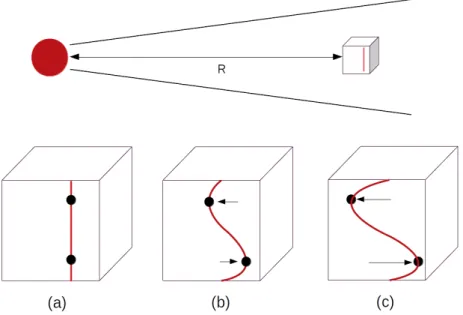
to fragmentation, which is thought to be one of the channels for the formation giant planet. Under the presence of the magnetic field, magnetorotational instability(MRI) may arise. The process that how this instability occurs is illustrated by Figure 2.4. Consider the vicinity of the point at a distance R co-rotating with the star, with two point masses well-coupled with the magnetic field. Under the perturbation, the two masses are then separated radially, and due to the Keplerian motion radial displacement causes subsequent angular separation. The
Figure 2.4: Illustration of the magnetorotational instability(MRI). (a) initially unperturbed state; (b) perturbation causes small radial displacement, resulting in angular displacement; (c) magnetic tension removes the angular momentum and further separates two elements.
magnetic tension then acts on and transfers angular momentum from the inner mass element to the outer one, which further enhances the radial displacement and lead to instability. Detailed magnetohydrodynamical(MHD) calculation and stability analysis showed that given any power-law angular velocity ⌦/ R q, if the condition q > 0 is fulfilled, arbitrarily weak magnetic field
can still induce this instability.
Other instabilities, such as purely hydrodynamical instability and shear instability, are also important in generation of turbulence and structure formation. The situation will be further complicated if solid is present and couples with the gas, while additional channel of instability, e.g. streaming instability, may emerge as a result of the angular momentum exchange between solid and gas.
2.2.5
Disk Dispersal
The total mass of the PPD is obviously not conserved: during the disk evolution the PPD continuously loses mass and eventually enters the gas-free stage after most of the gas is lost. The dominant channel of mass loss is the gas accretion onto the star. Taking the accretion rate to be the median of the observed value, which is 10 8M yr 1, one can estimate that the
disk has a lifetime in the order of million year. However, if the accretion is the only channel that contributes to the mass loss, the discrepancy between the theory and observation arises as the mass loss rate will be too low at the final stage of the disk. This contradicts the fact that disks in such stages have not been observed(Alexander et al., 2013). It is then reasonable to consider other means of mass removal which can produce a sharp cut-o↵ of surface density evolution rather than a tail. Based on this motivation, the two main candidates for mass loss are the photoevaporation and MHD winds.
16 Chapter 2. The Protoplanetary Disk
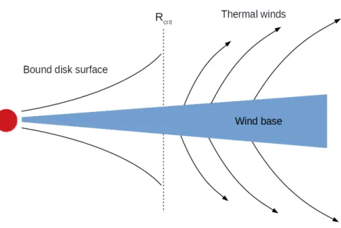
Figure 2.5: Illustration of the thermal winds launched due to photoevaporation.
Photoevaporation
Mass loss due to photoevaporation is caused by the thermal winds launched from the surface of the disk. The high-energy photons from the star or other sources can ionise the molecule on the surface of the disk and raise the temperature. When the thermal energy of the particle exceeds the gravitational potential energy, the particle will no longer remain bounded, resulting in thermal winds that carry matter away. To understand this e↵ect quantitatively, we define a critical distance Rcritat which the gas particle is able to escape. Careful calculations considering
wind structure and rotation show that
Rcrit ⇡ 0.2Rgrav, (2.62) where Rgrav = GM⇤ c2 s (2.63) is the distance when the thermal energy kBT is equal to the gravitational energy, and cs is the
sound speed of the gas. Figure 2.5 shows the illustrative picture of photoevaporation. Within the critical radius, the gas is bounded by the flared disk surface; beyond the critical radius, thermal winds were launched from the base, which carry away the mass at around sound speed. The mass loss rate per unit area, ˙⌃evap, can thus be expressed as
˙⌃evap ⇡ 2µmHn0cs, (2.64)
where µ is the mean molecular weight, n0 is the number density at the base and is a function
of distance R. Generally solving the radiative transfer equation is required to obtain n0(R).
radius Rin to the outer radius of the disk Rout: ˙ Mevap= Z Rout Rin 2⇡R ˙⌃evapdR. (2.65)
The photoevaporation e↵ect obviously depends on the energy of the photons, and the above analysis is mainly valid in the case of the extreme ultraviolet(EUV) photon. Under the flux of EUV photon, there will be a sharp ionising front separating the heated layer and the remaining cool part of the disk. In the case of the X-ray and far ultraviolet photons, the sharp front is absent, making the analytical modelling even harder. Given the flux of EUV to be , the mass loss rate estimated by Font et al. (2004) is
˙ Mevap⇡ 1.6 ⇥ 10 10 ✓ M⇤ M ◆1/2✓ 1041s 1 ◆1/2 M yr 1. (2.66) MHD Wind
The MHD wind is an alternative source of the mass loss, which can be launched by the magneto-centrifugal driving force in the presence of the magnetic field lines. To understand this e↵ect, we can first write down the Lorentz force per unit volume as
J⇥ B c = r ✓ B2 8⇡ ◆ +B· rB 4⇡ . (2.67)
Here J is the current density and B is the magnetic field. The first and second terms on the right-hand side are the magnetic pressure and tension, respectively. In the region close to the mid-plane of the disk, i.e., z ⌧ h where z is the height, the thermal pressure ⇢gc2s is larger than
the magnetic pressure B2/8⇡; however, as z increases thermal pressure drops due to decrease in
density, where magnetic pressure stays almost constant due to conservation of flux. Therefore, beyond a certain height the magnetic pressure will dominate over the thermal pressure and the wind is launched. The wind is then supported by the field line until the Alfv´en surface is reached, where kinetic energy density ⇢gv2 surpasses the magnetic energy density. Beyond this
boundary the wind will be strong enough to bend the field lines. Between where the wind is launched and the Alfv´en surface, the acceleration due to magnetic field is assumed to be nearly zero, which means J⇥ B ⇡ 0. This region is called the force-free region.
Compared to the thermal wind driven by photoevaporation, MHD wind depends only on the magnetic flux and thus can be launched at even very inner part of the disk, since it is not constrained by the star’s potential. The investigation on the coupling between these two e↵ects remains as an open question; nevertheless in reality the disk winds are more likely to be driven by both the photoevaporation and MHD e↵ect.
Chapter 3
Planetary Migration
A planet is never an isolated object: along its evolution history it keeps interacting gravita-tionally with its surroundings, including the PPD where it was born and the star that it was bound to. In this chapter we will review the various interactions between the planet and its surrounds, mainly the planet-disk interaction. This review basically follows Armitage (2010). When a planet is embedded in a PPD, it keeps exchanging of the angular momentum via gravitational torques and, as a result, migrates. This is called the planetary migration. The planetary migration is particularly important in considering the early evolution phase of a planetary system as it can significant change the planetary configuration in a short time-scale. Modelling the planetary migration requires the quantitative understanding the physical ori-gins of the torques arising from the non-axisymmetric structure of the disk. Here we follow the treatment of Goldreich & Tremaine (1979), which approached this problem by considering the linear perturbation of the gravitational potential followed by the responses of the disk in di↵erent resonant modes.
3.1
The Resonant Torques
Using the same mathematical formalism as Goldreich & Tremaine (1979), we use the cylindrical coordinate system (R, ✓, z). Let v0 = R⌦ˆe✓ and 0 be the unperturbed azimuthal velocity and
surface density, while v1 and 1 are the first order perturbations of the respective quantity.
We introduce an external perturbation potential 1(R, ✓, t) and denote the additional potential
perturbation due to 1 as 1D. The linearised hydrodynamical perturbation equations then
reduce to @v1 @t + (v0· r)v1+ (v1· r)v0 = r( 1+ D 1 + ⌘1), (3.1) @ 1 @t +r · ( 0v1) +r · ( 1v0) = 0, (3.2) 18
where ⌘1 = c2s0 ✓ 1 0 ◆ , (3.3) r2 D 1 = 4⇡G 1 (z). (3.4)
Here cs0 is the unperturbed sound speed, (z) is the Dirac delta function, and ⌘ is the enthalpy
related to the sound speed. Equations (3.1) and (3.2) are derived from the angular momentum conservation and mass conservation, respectively. Then by writing each perturbation variable in the form of X = X(R) exp i(m✓ !t) with m being an integer, the momentum conservation can be re-written as i(m⌦ !)v1,R 2⌦v1,✓ = d dR( 1+ D 1 + ⌘1), (3.5) 2Bv1,R+ i(m⌦ !)v1,✓ = im R ( 1+ D 1 + ⌘1), (3.6)
where v1,R and v1,✓ are ˆR and ˆ✓ components of v1. B is the Oort parameter defined as
B(R) = ⌦(R) +R 2
d⌦
dR, (3.7)
Solving v1,R and v1,✓ from the above equations, we obtain
v1,R = i D (m⌦ !) d dR + 2m⌦ R ( 1+ D 1 + ⌘1), (3.8) v1,✓ = 1 D 2B d dR + m R(m⌦ !) ( 1+ D 1 + ⌘1), (3.9) D = 2 (m⌦ !)2, (3.10)
where = 2pB(R)⌦(R) is the epicyclic frequency. We can then substitute the above solution to the mass conservation equation, and the resulting di↵erential equation shows that there will be singularities at both m⌦ ! = 0 and D = 0. These correspond to
1. Co-rotational resonance: ⌦(R) = !,
2. Lindblad resonance: m(⌦(R) !) =±(R).
In the case that the planet is the perturbation source, ! = ⌦p, where ⌦p is the angular velocity
of the planet. This means that the co-rotational resonance happens at the same R as the planet. For the Lindblad resonance, if the disk is Keplerian, ⌦(R) = (R), and
⌦p = ⌦(R) ✓ 1⌥ 1 m ◆ . (3.11)
20 Chapter 3. Planetary Migration
If the planet is in a circular orbit with semi-major axis ap,
ap3/2 = RL3/2 ✓ 1⌥ 1 m ◆ , (3.12) RL= ✓ 1⌥ 1 m ◆2/3 ap, (3.13)
where RL is the position that Lindblad resonance takes place. This shows that Lindblad
resonance can take place at multiple places. Further detailed calculation of the torques can be found in Goldreich & Tremaine (1979).
The modelling described above provides a unified framework for two di↵erent types of the migrations, namely the Type I and Type II migrations. We will review each of them in the following subsections.
3.2
Type I migration
The Type I migration happens when the planet mass is low so that the the disk structure can be approximately assumed to be unperturbed due to relatively weak planet-disk interaction. In this case the viscous torques dominates the local angular momentum transport around the planet, we can neglect the change of structure of the disk due to the planet’s gravitational torques and all the resonance modes are available. The total torque tot that is experienced by
the planet can be written as a summation of both the co-rotational and Lindblad torques
tot = X ( L,out+ C) = 1 X m=1 L,out+ 1 X m=2 L,in+ C. (3.14)
Here L,in and L,out are the Lindblad partial torques at inner and outer resonances and C is
the co-rotational torque.
The computation of the torque requires special mathematical expertise to solve the wave equa-tions, and this is usually done by performing numerical integrations. The solutions given by Tanaka et al. (2002) shows that given a planet in a circular orbit located at Rp and the disk
surface density profile d ln ⌃/d ln R = s, the Lindblad and corotational torques experienced by the planet can be approximated by:
L= (2.34 + 0.10s) 0, (3.15) C = (0.98 + 0.64s) 0, (3.16) 0 = ✓ Mp M⇤ ◆2✓ hp Rp ◆ 2 ⌃(Rp)R4p⌦2K(Rp), (3.17)
where Mp/M⇤ is the planet-star mass ratio, hp/Rp is the aspect ratio at the planet’s position
and ⌦K is the Keplerian angular velocity. More recent results with consideration of non-linear
horseshoe drag can be found in Paardekooper et al. (2010) and will be introduced in section 5.1.4. To translate the torque to the motion of planet, we can introduce an e-fold migration
timescale, and the methodology will be described in Section 5.1.1.
3.3
Type II migration
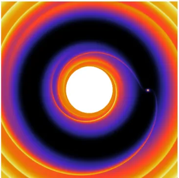
Figure 3.1: Gap carved by a giant planet, as shown by hydrodynamical simulation. Color coded according to the surface density. Credit: Dr. K. Kanagawa.
The Type II migration happens when the planet mass is high so that the viscous torques around the planet cannot compete with the strong gravitational torques exerted by the planet. As a result, the gas at the vicinity of the planet is repelled and a gap is formed since the vicious di↵usion cannot replenish the gas. The low density at the gap means that all the resonant modes that are close to the planet will be ine↵ective, and therefore the total inward migration torque is weaker compared to that of the Type I migration. In the classical picture of Type II migration, the planet keep removing the the angular momentum of the gas from the inner edge of the gap and adding the same amount of momentum to the outer edge, and thus the inward mass flow and angular momentum flow will be una↵ected as an unperturbed case without a planet. The planet will migrate inward at the same viscous speed as the gas, which we have already derived in Section 2.2.1, the equation (2.40):
vR =
3⌫
2R. (3.18)
Compared with Type I migration, Type II migration is much slower, which corresponds to a longer migration timescale. Following the same idea, we may think the time-scale to form a steady gap tgap is equal to the viscous di↵usion time derived in equation (2.47):
tgap=
h2
⌫ . (3.19)
22 Chapter 3. Planetary Migration
profile and the viscosity of the disk. We will consider the dependence of these parameters in details in Chapter 5.
The HL Tau system
In the previous chapters, we have already reviewed the basic properties of PPD and also inter-actions inside the disk, which can then be implemented numerically to perform the simulation. We are now one-step away from a complete picture of the simulation, and the last piece is the initial conditions. One of the highlights of this project is that we start from the realistic initial conditions that are deduced from the HL Tau system, a young star hosting a PPD in the Taurus star forming region. Being regarded as “an excellent example of a system just emerging from its protostellar cocoon” by Partnership et al. (2015), the HL Tau system is the first PPD observed to have the concentric ring and gap structure. Thanks to the high resolution imaging of ALMA, we are able to deduce and extract rich information from its disk structure and properties, such as the surface density profile, the gap structure and possible locations of the planets. In this chapter, we will review the observation of ALMA, the follow-up analysis and the pioneering work that links such observation to the evolution of multi-planetary system.
4.1
Disk Structure and Properties
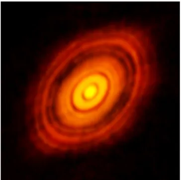
ALMA observed the HL Tau from October 2014 to November 2014. The dust continuum images were taken at three di↵erent bands, the Band 6(1.3 mm), Band 7(0.87 mm) and Band 3(2.9 mm). The achieved resolution ranged between 0.07500 to 0.02500, corresponding to 10 au to 3.5 au. One
can refer to Partnership et al. (2015) for the full technical details of the observation and data calibration. Figure 4.1 is the dust continuum image of HL Tau taken at Band 6(233 GHz). Kwon et al. (2015) used both the viscous accretion and power-law disk model to fit the con-tinuum data, and found out that the accretion model can fit better. Assuming the gas-to-dust ratio to be 100, the fitting result shows that the disk of HL Tau has a mass of 0.105(1) M , with inner edge at 8.78(19) au and outer edge(exponential cut-o↵) extended to 80.20(34) au. If the gas-to-dust ratio is assumed to be 100, the fitting result of its disk surface density can be expressed as ⌃g(R) = 5.66⇥ 10 4 ✓ R 80 au ◆0.2 exp " ✓ R 80 au ◆2.2# M au 2, (4.1)
where R is the cylindrical distance.
24 Chapter 4. The HL Tau system
Figure 4.1: The ALMA image of HL Tau (https://www.eso.org/public/images/eso1436a/).
The accretion rate of the HL Tau is estimated to be 8.7⇥ 10 8M yr 1. The upper limit of
viscosity ↵ can thus be estimated via accretion rate as
↵(R) = M˙
3⇡cs(R)h(R)⌃g(R)
. (4.2)
At R = 100 au, h ⇠ 10 au, ⌃g ⇠ 10 5M au 2. This gives the upper limit of the viscosity to be
10 2. Alternatively, viscosity can also be estimated from the dust settling, and the result is in
order of 10 4(Pinte et al., 2015).
4.2
Planetary signatures: the gap structure
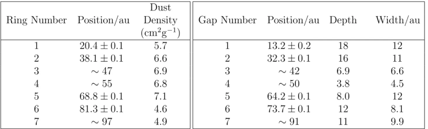
The most important accomplishment of Partnership et al. (2015) is the alternate bright and dark ring-like structure that can be clearly seen from Figure 4.1. In total seven rings and seven gaps were observed, and their respective positions and properties are summarised in Table 4.1. To avoid any confusion, we will follow the nomenclature that uses the term ‘ring’ to denote bright ring and ‘gap’ to denote the dark ring.
The discovery of the gaps deserves particular attention as it can potentially indicate the presence of giant planets. Although theories (e.g., Lin & Papaloizou, 1979; Goldreich & Tremaine, 1980; Crida et al., 2006) have long predicted that a giant planet inside a disk can gravitationally interact with its surroundings and create a gap by clearing its orbit, until Partnership et al. (2015) there was no direct proof to confirm the existence of such structures. On the other hand, alternative interpretations of the gap origin, including instability (e.g., Takahashi & Inutsuka, 2016) and snow lines (e.g., Zhang & Jin, 2015), are also possible. In this thesis, we take the assumption that the gaps are created by planets.
Dust Ring Number Position/au Density
(cm2g 1) 1 20.4± 0.1 5.7 2 38.1± 0.1 6.6 3 ⇠ 47 6.9 4 ⇠ 55 6.8 5 68.8± 0.1 7.1 6 81.3± 0.1 4.6 7 ⇠ 97 4.9
(a) Ring positions and dust opacity of HL Tau. Dust opacity corresponds to = 1 mm.
Gap Number Position/au Depth Width/au
1 13.2± 0.2 18 12 2 32.3± 0.1 16 11 3 ⇠ 42 6.9 6.6 4 ⇠ 50 3.8 4.5 5 64.2± 0.1 8.0 12 6 73.7± 0.1 12 8.1 7 ⇠ 91 11 9.9
(b) Gap positions and gap depth of HL Tau. Gap depth is the ratio of density at vicinity of the gap to the mini-mum density at the gap.
Table 4.1: Ring and gap properties of HL Tau (Partnership et al., 2015).
planet’s mass, the viscosity and the aspect ratio of the disk. The analytical estimates given by Kanagawa et al. (2015) show that this relation has the form
⌃min
⌃ = 1
1 + 0.04K. (4.3)
Here ⌃min is the minimum density at the bottom of the gap and ⌃ is the density at vicinity of
the gap. The dimensionless parameter K is expressed as
K = ✓ Mp M⇤ ◆2✓ hp Rp ◆ 5 ↵ 1. (4.4)
Using two-dimensional hydrodynamical simulations, Kanagawa et al. (2016) further obtained an empirical formula which gave the relation between the width of the gap g the planet’s
location Rp g Rp = 0.41 ✓ Mp M⇤ ◆1/2✓ hp Rp ◆ 3/4 ↵ 1/4, (4.5)
which yields the mass of the planet in terms of the gap width, aspect ratio and viscosity as Mp M⇤ = 2.1⇥ 10 3 ✓ g Rp ◆2✓ hp/Rp 0.05 ◆3/2⇣ ↵ 10 3 ⌘1/2 . (4.6)
The above equation can be used to estimate the mass of hidden planets in HL Tau. Given ↵ = 3⇥ 10 4 and the width of the respective gap, the fiducial values for the mass of the
innermost three planets are estimated as 0.77, 0.11, and 0.27 MJ when the mass of HL Tau is
26 Chapter 4. The HL Tau system
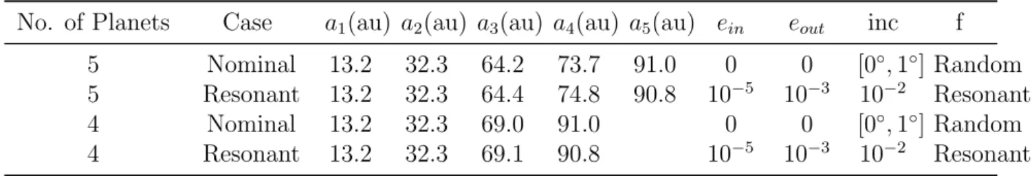
No. of Planets Case a1(au) a2(au) a3(au) a4(au) a5(au) ein eout inc f
5 Nominal 13.2 32.3 64.2 73.7 91.0 0 0 [0 , 1 ] Random 5 Resonant 13.2 32.3 64.4 74.8 90.8 10 5 10 3 10 2 Resonant 4 Nominal 13.2 32.3 69.0 91.0 0 0 [0 , 1 ] Random 4 Resonant 13.2 32.3 69.1 90.8 10 5 10 3 10 2 Resonant
Table 4.2: HL Tau initial conditions used by Simbulan et al. (2017).
4.3
Previous Study: Planetary Dynamics in HL Tau
System
We have seen that a large amount of information about the possible configuration of a young multi-planetary system is hidden inside the revolutionary ALMA image of HL Tau. Simbulan et al. (2017) took this idea and connected the HL Tau image to the initial conditions of planetary systems. In this pioneering work, they extracted the orbital information from the gaps of HL Tau and systematically examined the possible outcomes of its evolution using numerical simulations. The main focus of their research is to investigate whether the initial conditions extracted from the HL Tau can reproduce a diverse configurations of multi-planetary systems that have been observed, given the allowed ranges of free parameters.
Figure 4.2: An example evolution of a 5-planet system reproduced from the initial conditions specified by Simbulan et al. (2017). The planet will be removed if it is ejected from the system or collide with the hosting star/another planet. In this system, four planets are either ejected or collided with the star within 3.5⇥ 107yr, and only one planet remains.
The orbital initial conditions that were used by Simbulan et al. (2017) are summarised in Table 4.2. Since the total number of planets that HL Tau may host are unknown, they considered both the 4-planet and 5-planet cases. Each case was further divided into nominal and resonant cases: for nominal cases, the initial positions of the planets are basically assigned to be the
location of the ring; for resonant cases, the planetary systems are first allowed to enter the resonant states via a ‘warm-up’ test, and the real simulations will start after the resonance is reached. The mass of the planets are assumed to be equal: 1.1 MJ was set to be the mass of
each planet for the five-planet case and 4.7 MJ for the four-planet case. Particularly, the planet
mass for the four-planet case is larger than that of five-planet case since the planetary system is intentionally set to be dynamically unstable.
For each case, 100 instances with randomised phase angles were simulated and each instance was evolved up to 5 Gyr. Simulation results show that a significant fraction of planets were ejected for both five-planet and four-planet case, with some planets collided with the star or another planet. Figure 4.2 shows an example evolution of semi-major axis in a 5-planet system from initial conditions specified in Table 4.2. The surviving planets showed a diverse distribution of eccentricity, inclination and semi-major axis. Simbulan et al. (2017) also compared the results with the population of eccentric Jupiters, hot Jupiters and free-floating planets and they concluded that starting from the HL Tau initial conditions these populations can be reproduced.
We may realise that the assumption of the mass assignment that Simbulan et al. (2017) relies on is unnatural as it is intentionally biased towards unstable systems. Their work can be further extended by including the disk-planet interaction and mass accretion process, from which we can get more realistic initial conditions. As the HL Tau system is still young, it is possible that the disk-planet interaction can strongly shape the initial conditions before the disk dispersal. Further investigation can also show how the planet-disk interaction will a↵ect the stabilities as well as the diversity of the planetary systems after long time evolution.
Chapter 5
Methods
5.1
Theoretical framework
5.1.1
Equations of Motion
When the disk is present, in addition to the gravitational forces from the central star and other planets, the planet will experience additional forces due to the disk. Consider the forces acting on the i-th planet inside the gap of the disk, the equation of motion can be written as
¨ri = fgrav,i+ fa,i+ fe,i (5.1)
where ri is the position vector of the i-th planet. The f notations on the right hand side of
the equation are respective forces per unit mass exerting on the ith planet. We assume the planets to be co-planar in this research, and thus ri can be replaced by the position vector Ri
in cylindrical coordinate system. We will continue using capital R to denote the cylindrical position vector unless stated otherwise.
Gravity
The first term fgrav is the gravitational force exerted by the central star and other planets,
which takes the form(e.g.Murray & Dermott (2000)):
fgrav,i = G(M⇤+ Mi) Ri R3 i + k6=i X k GMk k Rk Ri k3 (Rk Ri) k6=i X k GMk R3 k Rk, (5.2)
where R = |R|. As in the previous chapters, we use symbol ⇤ to denote the central star and subscripts i, k as the indices of planets only. Since later we are going to perform the N -body simulation framework to carry out the simulations, in practice this term requires no special attention as it has been fully absorbed into the N -body integration framework.
Migration force
The second term fa,idenotes the force that drives the inwards-migration of planets. As discussed
in Section 3, a planet with index i embedded inside the disk experiences an e↵ective torque i
and migrates inwards. We define an e-fold migration timescale ⌧a,i
˙ai
ai ⌘
1 ⌧a,i
, (5.3)
where ai is the semi-major axis of the planet. To see the physical meaning of ⌧a,i, assuming
small eccentricity, we can write the migration velocity ˙Ri in terms of the torque and angular
momentum as: ˙ Ri = 2 i Li Ri, (5.4)
where Li = a2i⌦K,iMi is the orbital angular momentum, ⌦K,i is the Keplerian angular velocity
at Ri. For small eccentricity, |Ri| ⇡ ai, and equation (5.4) implies
⌧a,i=
Li
2 i
. (5.5)
To incorporate this migration into the N -body simulation, we implement the migration as an e↵ective force. Further di↵erentiation of equation (5.4) gives the acceleration:
¨ Ri = i ˙ Ri Mia2i⌦K,i = i Li ˙ Ri. (5.6)
Substituting equation (5.5) to (5.6) then the expression of fa,i is simply
fa,i = ¨Ri =
˙ Ri
2⌧a,i
. (5.7)
Eccentricity damping force
The disk also tends to circularise the planet’s orbit if the planet is in a eccentric orbit. Using the same spirit as equation 5.3, we define the eccentricity damping timescale, ⌧e,i and assume
the following linear relationship with ⌧a,i(Lee & Peale, 2002; Kley et al., 2004):
⌧e,i= ⌧a,i ✓ hi Ri ◆2 c, (5.8)
where h/R is the aspect ratio and c is a constant. Following Kanagawa et al. (2018), we take c = 1.282 in our simulation. We can then compute the eccentricity damping force as
fe,i = vi (1 e2 i)(3/2)⌧e,i + ˆli⇥ ˆRi r µ ai(1 e2i) 1 (3/2)⌧e,i , (5.9)
30 Chapter 5. Methods
5.1.2
Model of the Disk Structure Hosting Multiple Planets
In sections 2.2.1 and 2.2.2, we reviewed the classical picture of the disk surface density profile and derived the static solution. Since our simulations takes account of the change of surface density due to mass accretion onto the planets, we generalised equation (2.53) to the N -planet case to make it applicable in multi-planetary systems.
Consider the steady state with in total N planets located at Ri, i 2 {1, 2, ..., N}, and treat
each planet as a mass sink with accretion rate ˙Mi. Then the conservation of mass gives
˙ M (R) = 8 > > > > < > > > > : ˙ M⇤ (R < R1), ˙ M⇤+ n P i=1 ˙ Mi (Rn < R < Rn+1, n2 {1, 2, ...N 1}), ˙ M⇤+PN i=1 ˙ Mi (R > RN). (5.10)
Similarly, conservation of the angular momentum flow gives
˙ M (R)j(R) = 8 > > > > < > > > > : ˙ M⇤j⇤ (R < R1), ˙ M⇤j⇤ + n P i=1 ˙ Miji (Rn< R < Rn+1, n2 {1, 2, ...N 1}), ˙ M⇤j⇤ +PN i=1 ˙ Miji (R > RN), (5.11)
where ji = j(Ri) = R2i⌦i is the specific angular momentum. Now consider the case of when
Rn < R < Rn+1. Using the boundary conditions at R = Ri, we can solve equation (2.49) as
3⇡⌫j(R)⌃g(R) = ˙M j(r) M˙⇤j⇤ n X i ˙ Miji. (5.12)
Substituting equation 5.10 to the above equation, we have
⌃g(R) = ˙ M⇤ 3⇡⌫ ✓ 1 j⇤ j(R) ◆ + n X i=1 ˙ Mi 3⇡⌫ ✓ 1 ji j(R) ◆ = M˙⇤ 3⇡⌫ 1 r R⇤ R ! + n X i=1 ˙ Mi 3⇡⌫ 1 r Ri R ! . (5.13)
The above formula shows that given the positions of all the planets, the surface density at position R is specified by the accretion rate ˙Mi alone. We define the global accretion rate as
the sum of all the accretion rates: ˙ Mglob = ˙M⇤+ N X i=1 ˙ Mi (5.14)
Our simulation assumes that ˙Mglobis a constant. It can be seen from the next section that once
˙
Mglob and the planet system configuration are specified, the individual ˙Mi can be calculated
We adopt a simple exponential decaying model to account for the time dependence of the surface density due to disk dispersion:
⌃g(R, t) = ⌃g(R) exp ✓ t ⌧disk ◆ , (5.15)
where ⌧disk is the e-fold disk lifetime. Since the disk lifetime is very uncertain, we treat ⌧disk as
a global free parameter in the simulation and consider di↵erent values.
5.1.3
Accretion Model
Figure 5.1: The planetary accretion rate against the planet mass(single planet) at constant ⌃R=5 au. Parameters: ↵ = 4⇥ 10 3, Rp = 5.2 au, M⇤ = 1 M , ˙M⇤ = (2⇡) 110 8M yr˙ 1.
We follow Tanigawa & Tanaka (2016) to determine the accretion rate of each planet, ˙Mi. This
model shows the accretion rate is related to the accretion surface density(disk surface density at the planet’s accretion site) ⌃acc as
˙
Mi = Di⌃acc,i, (5.16)
where Di is the accretion area of the protoplanetary disk per unit time given by
Di = 0.29 ✓ hi Ri ◆ 2✓ Mi M⇤ ◆4/3 R2i⌦i. (5.17)
In the above, ⌦i is the angular velocity of the i-th planet, which may not be equal to ⌦K,i;
nevertheless we take the approximation that ⌦i ⇡ ⌦K,i. We also assume that the accretion