Vol. 60, No. 4, October 2017, pp. 461–478
AN ADAPTIVE COST-BASED SOFTWARE REJUVENATION SCHEME WITH NONPARAMETRIC PREDICTIVE INFERENCE APPROACH
Koichiro Rinsaka Tadashi Dohi
Kobe Gakuin University Hiroshima University
(Received July 15, 2016; Revised July 10, 2017)
Abstract This paper proposes an approach to estimate an optimal software rejuvenation schedule mini-mizing an expected total software cost per unit time. Based on a non-parametric predictive inference (NPI) approach, we derive the upper and lower bounds of the predictive expected software cost via the predictive survival function from system failure time data, and characterize an adaptive cost-based software rejuvena-tion policy, from the system failure time data with a right-censored observarejuvena-tion. In simularejuvena-tion experiments, it is shown that our NPI-based approach is quite useful to predict the optimal software rejuvenation time.
Keywords: Reliability, software rejuvenation, software aging, statistical estimation,
adaptive policy, non-parametric predictive inference, software cost model 1. Introduction
Software dependability is one of stringent requirements for present day applications, be-cause a huge economic loss or risk to human life can be be-caused by the consequences of software failure in some cases. While these requirements cannot be fulfilled in designing actual applications with non-trivial complexity, the reduction of software development cost is frequently requested in industry. This dilemma penalizes applying the classical design diversity techniques in software fault-tolerance, such as recovery block and N version pro-gramming, to the common application development. Instead, the environment diversity techniques to realize time redundancy in software operation receive considerable attention in recent years. In other words, since bug fixing is not always possible for continuously running software systems, patch release is becoming much popular to maintain software applications in operational phase. However, as reported in Gray and Siewiorek [22] and Grottke and Trivedi [23], most software failures are transient in nature and will disappear if the operation is retried later in slightly different context. These software bugs which cause transient failure are called Mandelbugs, and it is in general difficult to characterize their root origin. Among them, the aging-related bugs are frequently observed in real world, when software application executes continuously for long periods of time. The phenomenon that the aging-related bugs cause software to age due to the error conditions that accrue with time and/or load, is called software aging. Adams [3], Avritzer and Weyuker [4], Avritzer et al. [5], Castelli et al. [9], Grottke et al. [24], Tai et al. [38], Yurcik and Doss [44] report several aging phenomena in real software systems.
Software rejuvenation is a complementary approach to handle transient software failures caused by the aging-related bugs (Huang et al. [26]) which can be regarded as a preventive and proactive maintenance solution. It is one of software environment diversity techniques and involves stopping the running software occasionally, cleaning its internal state and restarting it. Typical examples of software rejuvenation are garbage collection, flushing
operating system kernel tables, reinitializing internal data structures, as well as retry, re-configuration, and reboot of systems. Since the seminal contribution by Huang et al. [26], a number of authors concern the problem how frequent software rejuvenation is triggered, because it has a tradeoff relationship between system down cost at failure and planned down cost by preventive rejuvenation. First, Huang et al. [26] propose a simple continuous-time Markov chain (CTMC) model with four states, i.e., initial robust (clean), failure probable, rejuvenation and failure states, to describe the stochastic behavior of a telecommunication billing application. They evaluate both the system unavailability and the operating cost in steady state under the random software rejuvenation schedule. Unfortunately, it is shown in Dohi et al. [15] that their CTMC assumption does not motivate to trigger software rejuve-nation. In Dohi et al. [15] and their subsequeent papers (e.g. see Danjou et al. [14], Dohi et al. [16–18]), it was shown that a sufficient condition for the existence of non-trivial software rejuvenation timing is that the transition probability from failure probable state to failure state has to be strictly increasing failure rate. In the above references, some semi-Markov models to describe the stochastic behavior of the telecommunication billing application are proposed. In addition to the stochastic modeling, statistical inference of the optimal soft-ware rejuvenation schedule is a challenging issue. Danjou et al. [14] and Dohi et al. [15–18] propose non-parametric estimation algorithms based on the empirical distribution to obtain the optimal software rejuvenation schedule from the complete sample of failure time data. If a sufficient number of samples of failure time data can be obtained, then the resulting estimate of the optimal software rejuvenation schedule asymptotically converges to the real but unknown optimal solution almost surely. Recently, Zhao et al. [45] apply the acceler-ated life testing technique by injecting memory leaks in their experiments and examine the above non-parametric estimation methods in importance sampling simulation. Rinsaka and Dohi [34] propose another non-parametric estimation algorithm based on the kernel density estimation (Duin [19], Parzen [31], Silverman [36]) to improve the estimation accuracy of the optimal software rejuvenation schedule with a small sample data.
Apart from the time-based optimal software rejuvenation schedule, some other stochastic models have been considered in the literature. Bao et al. [6, 7], Bobbio et al. [8], Okamura et al. [29], Wang et al. [42], Xie et al. [43] develop workload-based software rejuvenation schemes. Though system parameters and resource usage strongly affect the software aging, it is pointed out that the mechanism on aging for individual software-based system has not been still clear. In other words, since the aging-related bugs are not bridged to system workload explicitly, it may be difficult to apply the workload-based software rejuvenation to tolerate transient failures completely. Vaidyanathan and Trivedi [39] propose a heuristic prediction-based software rejuvenation scheme, where the workload in future is predicted by means of linear regression model. Pfening et al. [32] consider a server-type software system with degradation as a queueing system, and formulate as the Markov decision process. Garg et al. [21] take account of the presence of system failure caused by software aging and analyze the time-based optimal software rejuvenation schedule. This model is extended latter in Okamura et al. [27–30] by introducing the workload-based rejuvenation schedule and/or a more general arrival process of transactions. van Moorsel and Wolter [40] focus on the system restart and derive the optimal restart policies to rejuvenate a software system over a finite and an infinite operational period.
In this way, considerable attention has been paid to describe the relationship between software aging and software rejuvenation scheduling. However, it is still difficult to provide a statistically meaningful estimator of the software rejuvenation schedule, because system’s failure behavior in real world is regarded as a rare event, and a sufficient number of
time-to-failure data cannot be observed in the operational phase. The accelerated life testing technique by Zhao et al. [45] will be useful under experimental environments, but is not always applicable to the operational phase of software systems. Then the key challenge is to develop a prediction-based adaptive software rejuvenation scheme. Rinsaka and Dohi [33,35] use a non-parametric predictive inference (NPI) approach by Coolen and Yan [10] and Coolen-Schrijner and Coolen [11]. They focus on a periodic software rejuvenation model Garg et al. [20] and Suzuki et al. [37] and derive the optimal NPI-based software rejuvenation time maximizing the steady-state availability criterion. In fact, the NPI approaches have been applied to a number of reliability and maintenance problems (Coolen-Schrijner et al. [12], Coolen-Maturi and Coolen [13], Aboalkhai et al. [1, 2], Venkat et al. [41]). In this paper, we reconsider the seminal work in Dohi et al. [15], and derive the NPI-based optimal software rejuvenation policy which minimizes the expected total software cost per unit time. Our motivation to consider the cost model is to distinguish two types of down time occurred by preventive (planned) rejuvenation and system failure by introducing the cost component. Dissimilar to the fixed sample problem in Dohi et al. [15–17] and Zhao et al. [45], it predicts the one-stage look-ahead behavior of system failure and sequentially estimates the optimal software rejuvenation time in an adaptive way. Similar to Coolen-Schrijner and Coolen [11], we formulate the upper and lower bounds of the predictive expected total software cost per unit time using the predictive survival functions obtained from n system failure time data, and derive the optimal software rejuvenation policies for (n + 1)-st system failure. On the basis of original data together with a right-censored observation, we derive adaptive rejuvenation policies. In the simulation experiments, we carry out the sensitivity analysis of some model parameters, and show the usefulness of the adaptive NPI approach proposed in this paper.
2. Model Description
We here introduce the software rejuvenation model proposed by Dohi et al. [15], which is an extension of CTMC model by Huang et al. [26]. The model based on the semi-Markov process has the following four states:
State 0: highly robust state (normal operation state)
State 1: failure probable state
State 2: failure state
State 3: software rejuvenation state.
Here, State 1 means that the memory leakage is over a threshold or the system lapses from the highly robust state into an unstable state. Let Z be the random time interval when the highly robust state changes to the failure probable state, having the common probability distribution function Pr{Z ≤ t} = F0(t) with finite mean µ0(> 0). Just after the
state becomes the failure probable state, system failure may occur with positive probability. Without loss of generality, we assume that the random variable Z is observable during the system operation (Huang et al. [26]). Let X denote the failure time from State 1, having the probability distribution function Pr{X ≤ t} = Ff(t) and the survival function S(t) =
1− Ff(t) with finite mean λf (> 0). If the system failure occurs before triggering a software
rejuvenation, then the recovery operation starts immediately at that time. Otherwise the software rejuvenation is triggered. Let Y be the random repair time from the failure state, having the common probability distribution function Pr{Y ≤ t} = Fa(t) with finite mean
0
1
2
3
completion of
repair completion of rejuvenation
system failure rejuvenation state
change
Figure 1: Semi-Markovian transition diagram for a simple four-states model
after the system state makes a transition from State 0 to State 1. Denote the probability distribution function of the time to invoke the software rejuvenation and the probability distribution of the time to complete software rejuvenation by Fr(t) and Fc(t) (with mean
µc(> 0)), respectively. After completing the repair or the rejuvenation, the software system
becomes as good as new, and the software age is initiated at the beginning of the next highly robust state. Consequently, we define the time interval from the beginning of the system operation to the next one as one cycle, and the same cycle repeats again and again. It is noted that all the states in State 0 ∼ State 3 are regeneration points. The transition diagram for Model 1 is depicted in Figure 1. If we consider the time to software rejuvenation time as a constant t0, then it follows that
Fr(t) = U (t− t0) =
{
1 if t ≥ t0
0 otherwise, (2.1)
where U (·) is the unit step function. We call t0 (≥ 0) the software rejuvenation schedule
in this paper. Hence, the underlying stochastic process is a semi-Markov process with four regeneration states. Note that under the assumption that the sojourn times in all states are exponentially distributed, this model is reduced to Huang et al.’s Markov model (Huang et al. [26]). Let cs (> 0) denote the repair cost per unit time, and cp (> 0) denote the
software rejuvenation cost per unit time. The expected total software cost per unit time in the steady-state is given by
C(t0) = csµa[1− S(t0)] + cpµcS(t0) µ0+ µa[1− S(t0)] + µcS(t0) + ∫t0 0 S(t)dt . (2.2)
In order to motivate to derive the optimal software rejuvenation schedule, we need to assume that cs> cp and csµa > cpµc (see Dohi et al. [15]).
3. Nonparametric Predictive Inference
The non-parametric predictive inference (NPI) approach is a comprehensive method to es-timate the optimal preventive rejuvenation schedule sequentially. Let Xj (j = 1, . . . , n)
and X(1) < X(2) < · · · < X(n) be independent and identically distributed continuous
non-negative random variables and their order statistics, respectively. Similar to Coolen-Schrijner and Coolen [11], we introduce the well-known Hill’s assumptions (Hill [25]):
(A-1) Ties of the system failure time data have probability 0, i.e., x(i) ̸= x(j) given that
x
(0)x
(1)x
(2)x
(3)x
(n−1)x
(n)t
0S
X n+1(t
0)
0
1/(n+1)
2/(n+1)
1
n
/(n+1)
(n−1)/(n+1)
(n−2)/(n+1)
S
X n+1(t
0)
S
X n+1(t
0)
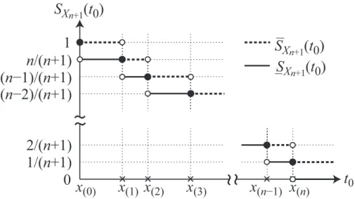
Figure 2: Configuration of predictive lower and upper survival functions
(A-2) Given x(j), j = 0, . . . , n, the probability that the next (n+1)-st system failure occurs
during Ij =
(
x(j), x(j+1)
)
is given by 1/(n + 1), where x(0) = 0 and x(n+1) → ∞ (or a
known upper limit of Xj), i.e., the predictive probability distribution has the mass part
of 1/(n + 1) for Ij =
(
x(j), x(j+1)
)
, j = 0, . . . , n.
More specifically when n system failure time data, x(1) < x(2) < · · · < x(n), are observed,
we obtain the predictive probability of (n + 1)-st system failure time interval Xn+1 by
Pr{Xn+1∈ ( x(j), x(j+1) )} = 1 n + 1, j = 0, . . ., n. (3.1)
From Equation (3.1), when t0 = x(j) (j = 0, . . . , n) the predictive survival function of Xn+1
is then given by SXn+1 ( x(j) ) = n− j + 1 n + 1 , j = 0, . . . , n + 1. (3.2)
It is worth noting in Equation (3.2) that the probability mass part of the survival function can be also defined only at the observation point x(j), but Hill’s assumptions do not put
any further restriction in the interval t0 ∈
(
x(j), x(j+1)
)
. Instead of the pointwise survival function, we consider the upper and lower bounds of predictive survival functions at an arbitrary time t0 between successive points
(
x(j), x(j+1)
)
. From an intuitive argument (see Figure 2), the greatest lower bound of the predictive survival function can be obtained by
SXn+1(x) = SXn+1 ( x(j+1) ) = n− j n + 1, x∈ (x(j), x(j+1)), j = 0, . . . , n. (3.3) Similarly, the least upper bound of the predictive survival function is derived by
SXn+1(x) = SXn+1 ( x(j) ) = n− j + 1 n + 1 , x∈ (x(j), x(j+1)), j = 0, . . . , n. (3.4) We call SXn+1(·) and SXn+1(·) the predictive lower and upper survival functions of Xn+1,
4. Optimal Software Rejuvenation Policies for Xn+1
4.1. Upper bound of predictive expected total software cost
In this section, the upper bound of predictive expected total software cost for (n + 1)-st sy1)-stem failure time interval, Xn+1, is derived via the lower bound of survival function
in Equation (3.3). Then we show that the optimal software rejuvenation schedule which minimizes the upper bound of predictive expected cost for Xn+1 can be attained at one of
the points x(j), j = 1, . . . , n. Let CXn+1(t0) denote the NPI-based upper bound of predictive
expected total software cost per unit time for Xn+1. By substituting the predictive lower
survival function in Equation (3.3) into Equation (2.2), we obtain the following lemma:
Lemma 4.1. CXn+1 ( x(j) ) = jcsµa+ (n− j + 1)cpµc (n+1)µ0+jµa+(n−j+1)µc+(n−j+1)x(j)+ ∑j−1 l=1 x(l) , j = 1, . . . , n + 1, (4.1) CXn+1(t0) = (j + 1)csµa+ (n− j)cpµc (n+1)µ0+(j +1)µa+(n−j)µc+(n−j)t0+ ∑j l=1x(l) , t0 ∈ ( x(j), x(j+1) ) , j = 0, . . . , n. (4.2)
As a special case of t0 = x(n+1)→ ∞, the NPI-based upper bound of predictive expected
total software cost is given by CXn+1 ( x(n+1) ) = csµa µ0 + µa+ n+11 ∑n l=1x(l) , (4.3) where E[Xn+1] = 1 n + 1 n ∑ l=1 x(l) (4.4)
is the lower bound of the expectation E[Xn+1]. It is obvious from Equation (3.3) that
SXn+1(t0) = 0 for ∀t0 > x(n). Hence, the upper bound of predictive expected total software
cost must be constant for t0 > x(n). Since SXn+1(t0) < SXn+1(x(n)) for t0 > x(n) from
Equations (4.1) and (4.2), it is found that t0 (> x(n)) does not minimize the upper bound
of predictive expected total software cost.
Lemma 4.2. For t0 ∈
(
x(j), x(j+1)
)
(j = 0, . . . , n− 1), the function CXn+1(·) is continuous
and monotonically decreasing in t0. Especially, CXn+1(·) is left-continuous at x(j) (j =
1, . . . , n) and each x(j) is a local minimum solution.
From Lemma 4.1 and Lemma 4.2, we obtain the following theorem on the optimal soft-ware rejuvenation policy for Xn+1 which minimizes the upper bound of predictive expected
total software cost.
Theorem 4.1. The minimum value of upper bound of predictive expected total software
4.2. Lower bound of predictive expected total software cost
Next, we derive the lower bound of predictive expected cost per unit time via the upper bound of survival function in Equation (3.4). Then we show that the optimal software rejuvenation schedule which minimizes the lower bound of predictive expected total software cost for Xn+1 can be attained at one of the points x−(j) (j = 1, . . . , n), where x−(j) is the left
limit of x(j). Let CXn+1(t0) be the NPI-based lower bound of predictive expected total
software cost. By substituting the predictive upper survival function in Equation (3.4) into the expected total software cost function in Equation (2.2), we have the following results.
Lemma 4.3. CXn+1(x(j) ) = jcsµa+ (n− j + 1)cpµc (n + 1)µ0+ jµa+ (n− j + 1)µc+ (n− j + 1)x(j)+ ∑j l=1x(l) j = 1, . . . , n + 1, (4.5) CXn+1(t0) = jcsµa+ (n− j + 1)cpµc (n + 1)µ0+ jµa+ (n− j + 1)µc+ (n− j + 1)t0+ ∑j l=1x(l) t0 ∈ (x(j), x(j+1)), j = 0, . . . , n. (4.6) Lemma 4.4. For t0 ∈ ( x(j), x(j+1) )
(j = 1, . . . , n), the function CXn+1(·) is continuous and monotonically decreasing in t0. Especially, CXn+1(·) is right-continuous at x(j), j = 1, . . . , n
and each x−(j) is a local minimum solution.
Theorem 4.2. The minimum value of lower bound of predictive expected total software
cost, CXn+1(·), can be attained at one of the points x−(j), j = 1, . . . , n.
In the case of t0 = x(n+1)→ ∞, the NPI-based lower bound of predictive expected total
software cost is given by CX n+1 ( x(n+1) ) = jcsµa (n + 1)µ0+ (n + 1)µa+ ∑n+1 l=1 x(l) = 0. (4.7)
In other words, as long as the upper bound of x(n+1) is infinite, the estimate of optimal
software rejuvenation schedule always becomes ˆt∗0 → ∞. In the plausible case where x(n+1)
is bounded and takes the value r, the upper bound of E[Xn+1] is given by
E[Xn+1] = 1 n + 1 ( n ∑ j=1 x(j)+ r ) . (4.8)
Then, comparing CXn+1(t∗0) with CXn+1(r−), where ˆt∗0 is the minimizer of lower bound of predictive expected total software cost, an estimate of the software rejuvenation schedule can be determined. Even when r is bounded but unknown, it is possible to calculate a critical value r∗ which satisfies CXn+1(t∗0) = CXn+1(r−). If r ≤ r∗, then the software rejuvenation schedule is given by ˆt∗0 otherwise it is always optimal not to invoke the software rejuvenation.
Table 1: Upper and lower bounds of predictive expected total software cost for X5+1 x(1) x(2) x(3) x(4) x(5) 1288 2087 2536 2882 3402 CX5+1(x(j)) 0.015480 0.014227 0.015549 0.017443 0.019387 CX5+1(x−(j)) 0.009423 0.009267 0.010534 0.012076 0.013428 4.3. Illustrative example 1
For better understanding, we give a simple example to derive the optimal software rejuve-nation time. Let
Tup,n+1∗ = argminCXn+1(t0) and T
−∗
low,n+1 = argminCXn+1(t0) (4.9)
denote the optimal software rejuvenation schedules corresponding to minimization of CXn+1
(t0) and CXn+1(t0), respectively. Suppose that n = 5 ordered samples of failure times are
available; 1288, 2087, 2536, 2882, 3402. The model parameters are fixed as µ0 = 240,
µa= 0.5, µc = 0.16, cs = 100, cp = 90. Table 1 presents the five failure time data, and the
resulting upper and lower bounds of the predictive expected total software cost, CX5+1(x(j))
and CX5+1(x−(j)) for X5+1. In this case, we have Tup,n+1∗ = Tlow,n+1−∗ = x(2) = 2087 with
CX5+1(2087) = 0.014227 and CX5+1(2087−) = 0.009267. The critical value of r∗ is given by
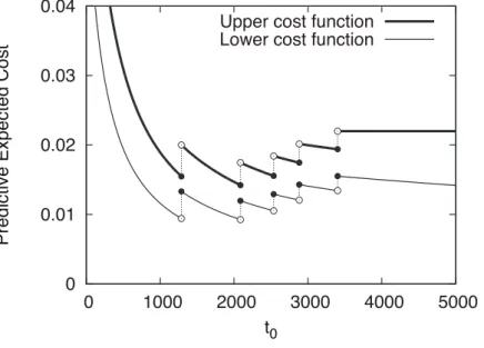
14892. Figure 3 is a plot of upper and lower functions of predictive expected total software cost.
As we will show in the latter discussion, Monte Carlo simulation experiments clarify the fact that Tup,n+1∗ is almost equal to Tlow,n+1−∗ in many cases. Even if Tup,n+1∗ differs from Tlow,n+1−∗ , Tup,n+1∗ can be regarded as the optimal software rejuvenation schedule from a viewpoint of an absolute error average against the theoretical minimum cost. Rinsaka and Dohi [33] investigate the above NPI-based software rejuvenation policies under a different dependability criterion and apply the real data analysis of a web server system.
0 0.01 0.02 0.03 0.04 0 1000 2000 3000 4000 5000 Pre d ict ive Exp e ct e d C o st t0
Upper cost function Lower cost function
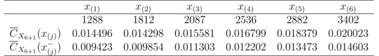
Table 2: Upper and lower bounds of predictive expected total software cost for X6+1
x(1) x(2) x(3) x(4) x(5) x(6)
1288 1812 2087 2536 2882 3402
CX6+1(x(j)) 0.014496 0.014298 0.015581 0.016799 0.018379 0.020023
CX6+1(x−(j)) 0.009423 0.009854 0.011303 0.012202 0.013473 0.014603
5. Adaptive Software Rejuvenation Prediction
We here consider an adaptive software rejuvenation schedule for (n + 2)-nd system failure. More precisely, after the optimal preventive rejuvenation schedule Tn+1∗ (= Tup,n+1∗ ) for (n + 1)-st system failure is triggered, we predict the next software rejuvenation schedule for (n + 2)-nd system failure from n + 1 system failure data or a right-censored observation at Tup,n+1∗ . This problem has not been considered in Rinsaka and Dohi [33] and gives a useful prediction scheme of the software rejuvenation.
5.1. Case of system failure before Tup,n+1∗
When the (n+1)-st system failure occurs before Tup,n+1∗ , the results obtained in the section 4 can be used as n := n + 1. In Example 1, we have T5+1∗ = 2087 for X5+1. Suppose that
6th failure occurs at 1812. Table 2 presents the six failure time data, and the upper and lower bounds of the predictive expected total software cost, CX6+1(x(j)) and CX6+1(x−(j)) for
X6+1. From Table 2, we have Tup,6+1∗ = Tlow,6+1−∗ = x(2) = 1812 with CX6+1(1812) = 0.014298
and CX6+1(1812−) = 0.009854. Hence, acquisition of the 6th failure time data hastens the optimal software rejuvenation schedule.
5.2. Case of rejuvenation at Tup,n+1∗
In the case where (n + 1)-st system failure time is greater than Tup,n+1∗ , namely the software system is preventively rejuvenated at time Tup,n+1∗ , the relevant data set consists of the n original system failure times together with a right-censored observation. Note that the right-censoring time is always equal to one of the n system failure times. We assume that the software rejuvenation was actually taken place at an x(k), k = 1, . . . , n, when the upper
predictive expected total software cost function was used. Then we consider an adaptive software rejuvenation schedule for (n + 2)-nd system failure time interval, Xn+2. Following
Coolen and Yan [10], the predictive survival function for the random lifetime Xn+2 is given
by SXn+2 ( x(j) ) = n + 2− j n + 2 , j = 0, . . . , k, (5.1) SXn+2 ( x(j) ) = (n + 2− k) (n + 1 − j) (n + 2) (n + 1− k) , j = k + 1, . . . , n + 1. (5.2) Similar to Section 4, the lower and upper survival functions at an arbitrary time between successive points (x(j), x(j+1) ) can be defined by SXn+2(x) = SXn+2 ( x(j+1) ) = n + 1− j n + 2 , x∈(x(j), x(j+1) ) , j = 0, . . . , k− 1, (5.3) SXn+2(x) = SXn+2 ( x(j+1) ) = (n + 2− k) (n − j) (n + 2) (n + 1− k), x∈(x(j), x(j+1) ) , j = k, . . . , n, (5.4)
SXn+2(x) = SXn+2 ( x(j) ) = n + 2− j n + 2 , x∈(x(j), x(j+1) ) , j = 0, . . . , k, (5.5) SXn+2(x) = SXn+2 ( x(j) ) = (n + 2− k) (n + 1 − j) (n + 2) (n + 1− k) , x∈(x(j), x(j+1) ) , j = k + 1, . . . , n. (5.6)
Let CXn+2(x(j)) and CXn+2(x(j)) denote the NPI-based upper and lower bounds of
predic-tive expected total software cost for Xn+2. The following lemma is derived by substituting
the predictive lower survival functions in Equations (5.3) and (5.4) into the expected total software cost function in Equation (2.2).
Lemma 5.1. The upper bound of predictive expected total software cost per unit time for Xn+2 is given by CXn+2 ( x(j) ) = jcsµa+ (n + 2− j)cpµc (n + 2)µ0+ jµa+ (n + 2− j)µc+ (n + 1− j)x(j)+ ∑j l=1x(l) , t0 = x(j), j = 1, . . . , k, (5.7) CXn+2 ( x(j) ) = Φ1 ( x(j) ) Ψ1 ( x(j) ), t0 = x(j), j = k + 1, . . . , n + 1, (5.8) CXn+2(t0) = (1 + j)csµa+ (n + 1− j)cpµc (n + 2) µ0+ (1 + j) µa+ (n + 1− j) µc+ ∑j l=1x(l)+ (n + 1− j) t0 , t0 ∈ ( x(j), x(j+1) ) , j = 0, . . . , k− 1, (5.9) CXn+2(t0) = Φ2(t0) Ψ2(t0) , t0 ∈ ( x(j), x(j+1) ) , j = k, . . . , n, (5.10) where Φ1 ( x(j) ) = (jn + 2j− k − jk)csµa+ (n + 2− k)(n + 1 − j)cpµc, (5.11) Ψ1 ( x(j) ) = (n + 2)(n + 1− k)µ0+ (jn + 2j− k − jk)µa+ (n + 2− k)(n + 1 − j)µc + (n + 2− k) j ∑ l=1 x(l)− k−1 ∑ l=1 x(l)+ (n + 2− k)(n − j)x(j), (5.12) Φ2(t0) = (jn + 2j− k − jk)csµa+ (n + 2− k)(n − j)cpµc, (5.13) Ψ2(t0) = (n + 2)(n + 1− k)µ0+ (jn + 2j− k − jk)µa+ (n + 2− k)(n − j)µc + (n + 2− k) j ∑ l=1 x(l)− k−1 ∑ l=1 x(l)+ (n + 2− k)(n − j)t0. (5.14)
The lower bound of predictive expected total software cost per unit time for Xn+2 is also
obtained by substituting the upper survival functions in Equations (5.5) and (5.6) into the expected total software cost function in Equation (2.2).
Lemma 5.2. The lower bound of predictive expected total software cost per unit time for Xn+2 is given by CX n+2 ( x(j) ) = jcsµa+ (n + 2− j)cpµc (n + 2) µ0+ jµa+ (n + 2− j) µc+ (n + 2− j) x(j)+ ∑j l=1x(l) , t0 = x(j), j = 1, . . . , k, (5.15) CXn+2(x(k+1) ) = Φ3 ( x(k+1) ) Ψ3 ( x(k+1) ), t0 = x(k+1), (5.16) CXn+2(x(j) ) = Φ4 ( x(j) ) Ψ4 ( x(j) ), t0 = x(j), j = k + 2, . . . , n + 1, (5.17) CXn+2(t0) = Φ5(t0) Ψ5(t0) , t0 ∈ ( x(j), x(j+1) ) , j = 0, . . . , k, (5.18) CX n+2(t0) = Φ6(t0) Ψ6(t0) , t0 ∈ ( x(j), x(j+1) ) , j = k + 1, . . . , n, (5.19) where Φ3 ( x(k+1) ) = (n + 2 + kn− k2)csµa+ (n + 2− k)(n − k)cpµc, (5.20) Ψ3 ( x(k+1) ) = (n + 2)(n + 1− k)µ0+ ( n + 2 + kn− k2)µa+ (n + 2− k)(n − k)µc + (n + 1− k)2x(k+1)+ (n + 1− k) k+1 ∑ l=1 x(l), (5.21) Φ4 ( x(j) ) = (jn + 2j− k − jk)csµa+ (n + 2− k)(n + 1 − j)cpµc, (5.22) Ψ4 ( x(j) ) = (n + 2)(n + 1− k)µ0+ (jn + 2j− k − jk)µa+ (n + 2− k)(n + 1 − j)µc + (n + 1− k) j ∑ l=1 x(l)+ j ∑ l=k+1 x(l)+ (n + 2− k)(n + 1 − j)x(j), (5.23) Φ5(t0) = jcsµa+ (n + 2− j)cpµc, (5.24) Ψ5(t0) = (n + 2)µ0 + jµa+ (n + 2− j)µc+ j ∑ l=1 x(l)+ (n + 2− j)t0, (5.25) Φ6(t0) = (jn + 2j− k − jk)csµa+ (n + 2− k)(n + 1 − j)cpµc, (5.26) Ψ6(t0) = (n + 2)(n + 1− k)µ0+ (jn + 2j− k − jk)µa+ (n + 2− k)(n + 1 − j)µc + (n + 1− k) j ∑ l=1 x(l)+ j ∑ l=k+1 x(l)+ (n + 2− k)(n + 1 − j)t0. (5.27)
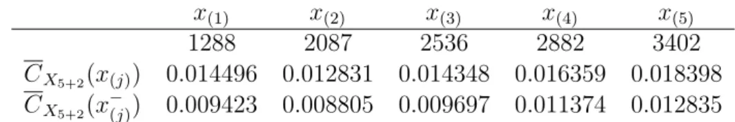
Table 3: Upper and lower bounds of predictive expected total software cost for X5+2
x(1) x(2) x(3) x(4) x(5)
1288 2087 2536 2882 3402
CX5+2(x(j)) 0.014496 0.012831 0.014348 0.016359 0.018398
CX5+2(x−(j)) 0.009423 0.008805 0.009697 0.011374 0.012835
In a fashion similar to the argument on Xn+1, we show that t0 > x(n) does not minimize
the upper bound of the predictive expected total software cost for Xn+2.
Lemma 5.3. (a) For t0 ∈
(
x(j), x(j+1)
)
(j = 0, . . . , n− 1), the function CXn+2(·) is
contin-uous and monotonically decreasing in t0. Especially, CXn+2(·) is left-continuous at x(j),
j = 1, . . . , n and each x(j) is a local minimum solution.
(b) For t0 ∈
(
x(j), x(j+1)
)
(j = 0, . . . , n), the function CXn+2(·) is continuous and mono-tonically decreasing in t0. Especially, CXn+2(·) is right-continuous at x(j) (j = 1, . . . , n)
and each x−(j) is a local minimum solution.
Theorem 5.1. (a) The minimum value of upper bound of predictive expected total
soft-ware cost per unit time, CXn+2(·), for Xn+2 can be attained at one of the points
x(j) (j = 1, . . . , n).
(b) The minimum value of lower bound of predictive expected cost per unit time, CXn+2(·), for Xn+2 can be attained at one of the points x−(j) (j = 1, . . . , n).
5.3. Illustrative example 2
Let
Tup,n+2∗ = argminCXn+2(t0) and T
−∗
low,n+2 = argminCXn+2(t0) (5.28)
denote the optimal software rejuvenation schedules corresponding to minimization of CXn+2
(t0) and CXn+2(t0), respectively. In Example 1, the optimal software rejuvenation schedule
has been estimated as Tup,5+1∗ = x(2) = 2087. Suppose that the (n + 1)-st system failure
time is right-censored at Tup,5+1∗ = 2087. Table 3 presents the five failure time data, and the upper and lower bounds of the predictive expected total software cost for X5+2. From
Table 3, we have Tlow,5+2∗ = Tlow,5+2−∗ = x(2) = 2087 with CX5+2(2087) = 0.012831 and
CX5+2(2087−) = 0.008805. Hence, the acquisition of right-censored time data does not change the optimal software rejuvenation schedule for Xn+2. This will be verified again in
simulation experiments in Section 6. From the simulation experiments we will show that Tup,n+2∗ works better in terms of an absolute error average with the theoretical minimum expected cost.
6. Simulation Experiments
Through simulation experiments, we compare the NPI-based optimal software rejuvenation schedule with the theoretically optimal solution, and verify the validity of the proposed NPI-based adaptive approach. Suppose that the random variable, X, obeys the Weibull distribution:
Ff(t) = 1− e−(t/θ)
γ
, γ > 0, θ > 0. (6.1)
In Table 4 we summarize the parameter setting, theoretical optimal software rejuvenation schedule and its associated minimum expected cost.
Table 4: Parameter setting, theoretical optimal software rejuvenation schedule and its as-sociated minimum expected cost
Case γ θ λf SD[X] µ0 µa µc cs cp t∗0 C(t∗0)
Case I 1.5 2215.46 2000.00 1357.93 240.00 0.50 0.16 100 90 1573.74 0.0203108 Case II 2.0 2256.76 2000.00 1045.45 240.00 0.50 0.16 100 90 1240.06 0.0173332 Case III 4.0 2206.53 2000.00 561.09 240.00 0.50 0.16 100 90 1266.56 0.0122037
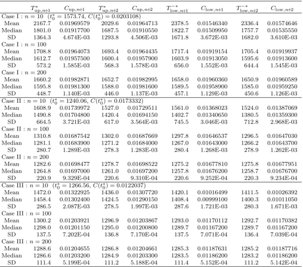
Table 5: Simulation results
Tup,n+1∗ Cup,n+1 Tup,n+2∗ Cup,n+2 Tlow,n+1−∗ Clow,n+1 Tlow,n+2−∗ Clow,n+2
Case I : n = 10 (t∗0= 1573.74, C(t∗0) = 0.0203108)
Mean 2167.7 0.01969579 2029.6 0.01964713 2378.5 0.01546340 2336.4 0.01574646 Median 1801.0 0.01917700 1687.5 0.01910550 1822.7 0.01509950 1757.7 0.01535550 SD 1364.3 4.674E-03 1293.8 4.506E-03 1671.8 3.672E-03 1682.0 3.610E-03 Case I : n = 100
Mean 1708.8 0.01964073 1693.4 0.01964435 1717.4 0.01919154 1705.4 0.01919937 Median 1612.7 0.01957500 1600.4 0.01957900 1603.9 0.01913050 1595.6 0.01913600 SD 573.2 1.585E-03 568.3 1.578E-03 656.0 1.552E-03 644.4 1.545E-03 Case I : n = 200
Mean 1660.2 0.01982871 1652.7 0.01982995 1658.0 0.01960360 1650.9 0.01960589 Median 1595.8 0.01981300 1588.0 0.01981600 1589.5 0.01958900 1585.0 0.01959250 SD 448.7 1.140E-03 446.0 1.137E-03 457.1 1.129E-03 450.6 1.126E-03 Case II : n = 10 (t∗0= 1240.06, C(t∗0) = 0.0173332)
Mean 1608.9 0.01739972 1527.0 0.01729511 1561.0 0.01368023 1524.0 0.01387069 Median 1490.8 0.01704800 1420.4 0.01694150 1402.7 0.01340650 1380.5 0.01359300 SD 664.5 3.721E-03 617.0 3.564E-03 745.5 3.046E-03 712.8 2.968E-03 Case II : n = 100
Mean 1310.8 0.01687542 1302.0 0.01687669 1297.8 0.01646537 1296.5 0.01647030 Median 1281.1 0.01683900 1271.2 0.01684000 1267.0 0.01643000 1266.2 0.01643700 SD 280.7 1.289E-03 278.3 1.283E-03 280.4 1.268E-03 278.9 1.262E-03 Case II : n = 200
Mean 1282.6 0.01698477 1278.7 0.01698522 1275.2 0.01677810 1275.8 0.01677951 Median 1264.8 0.01697000 1261.0 0.01697200 1257.8 0.01676200 1258.7 0.01676700 SD 220.9 9.329E-04 220.6 9.310E-04 220.6 9.252E-04 220.3 9.234E-04 Case III : n = 10 (t∗0= 1266.56, C(t∗0) = 0.0122037)
Mean 1472.0 0.01322925 1436.0 0.01307720 1420.1 0.01016499 1411.5 0.01026392 Median 1458.4 0.01302400 1424.5 0.01290150 1408.4 0.00999100 1400.3 0.01011050 SD 286.5 2.087E-03 278.5 1.997E-03 287.6 1.721E-03 280.3 1.671E-03 Case III : n = 100
Mean 1300.2 0.01203921 1296.9 0.01203867 1293.0 0.01170112 1292.7 0.01170382 Median 1298.0 0.01201150 1295.0 0.01200800 1289.7 0.01167200 1289.7 0.01167200 SD 137.5 7.202E-04 136.8 7.170E-04 137.5 7.071E-04 136.4 7.039E-04 Case III : n = 200
Mean 1288.6 0.01204655 1286.8 0.01204661 1285.3 0.01187631 1285.2 0.01187716 Median 1286.6 0.01203200 1284.9 0.01203300 1283.5 0.01186200 1283.2 0.01186200 SD 111.4 5.199E-04 111.2 5.188E-04 111.4 5.152E-04 111.2 5.142E-04
Table 5 shows the simulation results, where 10,000 simulations were performed for each case. We can observe from Table 5 that the means and medians of estimated optimal soft-ware rejuvenation schedules, Tup,n+1∗ and Tlow,n+1−∗ , for Xn+1 are greater than the theoretical
solution t∗0. As the number of failure time data increases, the means and the medians of estimated optimal preventive rejuvenation schedules gradually approach to t∗0, while the standard deviations (SDs) of Tup,n+1∗ and Tlow,n+1−∗ become smaller. For Xn+2, the means and
medians of Tlow,n+2∗ and Tup,n+2−∗ also tend to become larger than the theoretical solution. Similar results as for Xn+1 can be observed about the SDs of Tlow,n+2∗ and Tup,n+2−∗ . We can
also observe from Table 5 that the mean and the median of Tlow,n+2∗ are closer to t∗0 than Tlow,n+1∗ .
Table 6 shows the number of times that the upper preventive rejuvenation schedule accords with lower one. It is observed from Table 6 that these two estimates are in agreement
Table 6: Number of times that upper schedule accords with lower one
Tup,n+1∗ = Tlow,n+1−∗ Tup,n+2∗ = Tlow,n+2−∗
n 10 100 200 10 100 200
Case I 8385 9670 9830 8444 9776 9896
Case II 8775 9595 9700 9202 9817 9874 Case III 8948 9563 9746 9460 9772 9863
Table 7: Absolute error averages of upper and lower expected total software cost
∆up,n+1 ∆up,n+2 ∆low,n+1 ∆low,n+2 Case I
n = 10 3.746E-03 3.617E-03 5.344E-03 5.090E-03 n = 100 1.399E-03 1.392E-03 1.573E-03 1.565E-03 n = 200 9.978E-04 9.950E-04 1.081E-03 1.078E-03
Case II
n = 10 2.921E-03 2.799E-03 4.128E-03 3.945E-03 n = 100 1.107E-03 1.101E-03 1.261E-03 1.253E-03 n = 200 7.976E-04 7.960E-04 8.733E-04 8.711E-04 Case III
n = 10 1.774E-03 1.668E-03 2.316E-03 2.216E-03 n = 100 5.961E-04 5.937E-04 7.115E-04 7.085E-04 n = 200 4.354E-04 4.344E-04 4.944E-04 4.931E-04
Table 8: Number of right-censored observations in 10,000 simulations
n = 10 n = 100 n = 200
Case I 4545 5216 5333
Case II 6104 7125 7252
Case III 7932 8815 8874
in many cases, and a rate in agreement for Xn+2 tends to become greater than that for
Xn+1. Table 7 presents the absolute error averages of lower and upper expected total
software cost, where, for example, ∆up,n+1 means the absolute error average of the upper
predictive expected total software cost for Xn+1 against the theoretical optimal solution. We
can observe from Table 7 that ∆up,n+1 and ∆up,n+2 are smaller than ∆low,n+1 and ∆low,n+2,
respectively. Hence, Tup,n+1∗ and Tup,n+2∗ are the better as the optimal software rejuvenation schedules from a viewpoint of the absolute error average against the theoretical optimal solution. We can also observe that ∆up,n+1> ∆up,n+2 for all cases. Therefore, our adaptive
preventive rejuvenation schedule can estimate the expected total software cost with higher accuracy.
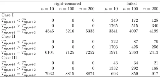
Table 8 shows the number of right-censored observations in 10,000 simulations, where Tn+1∗ = Tup,n+1∗ is used for optimal software schedule for Xn+1. As the shape parameter
of the Weibull distribution becomes larger, or as the number of data becomes larger, the number of times of software rejuvenation becomes larger. We show in Table 9 the number of times that optimal preventive rejuvenation schedule is increasing or decreasing. It is observed that the right-censored observation for Xn+1 does not change the next preventive
rejuvenation schedule. In the case where the system failure time is observed, on the other hand, the next schedule may not change or may change in both directions.
Table 9: Number of times that optimal software rejuvenation schedule is increasing or decreasing right-censored failed n = 10 n = 100 n = 200 n = 10 n = 100 n = 200 Case I Tup,n+1∗ < Tup,n+2∗ 0 0 0 349 172 128 Tup,n+1∗ > Tup,n+2∗ 0 0 0 1765 515 340 Tup,n+1∗ = Tup,n+2∗ 4545 5216 5333 3341 4097 4199 Case II Tup,n+1∗ < Tup,n+2∗ 0 0 0 222 87 79 Tup,n+1∗ > Tup,n+2∗ 0 0 0 1703 425 256 Tup,n+1∗ = Tup,n+2∗ 6104 7125 7252 1971 2363 2413 Case III Tup,n+1∗ < Tup,n+2∗ 0 0 0 43 34 21 Tup,n+1∗ > Tup,n+2∗ 0 0 0 1332 292 188 Tup,n+1∗ = Tup,n+2∗ 7932 8815 8874 693 859 917 7. Conclusions
In this paper, we have developed the NPI-based adaptive software rejuvenation schedule which minimizes the predictive expected cost per unit time. Under the Hill’s assumptions, we have derived the optimal software rejuvenation policies for (n + 1)-st system failure. Based on the n system failure time data together with the right-censored observation, we have adaptively derived the optimal software rejuvenation policies for (n + 2)-nd system failure. Through simulation experiments, it has been found that the NPI-based software rejuvenation policy can reduce the absolute error averages of the predictive expected total software cost against the theoretically optimal solution. This result implies the usefulness of our adaptive non-parametric predictive inference approach proposed in this paper.
References
[1] A.M. Aboalkhair, F.P.A. Coolen and I.M. MacPhee: Nonparametric predictive reliabil-ity of series of voting systems. European Journal of Operational Research, 226 (2013), 77–84.
[2] A.M. Aboalkhair, F.P.A. Coolen and I.M. MacPhee: Nonparametric predictive infer-ence for reliability of a k-out-of-m: G system with multiple component types. Reliability Engineering and System Safety, 131 (2014), 298–304.
[3] E. Adams: Optimizing preventive service of the software products. IBM Journal of Research & Development, 28 (1984), 2–14.
[4] A. Avritzer and E.J. Weyuker: Monitoring smoothly degrading systems for increased dependability. Empirical Software Engineering, 2 (1997), 59–7.
[5] A. Avritzer, A. Bondi, M. Grottke, E.J. Weyuker and K.S. Trivedi: Performance as-surance via software rejuvenation: monitoring, statistics and algorithms. Proceedings of the 36th Annual IEEE/IFIP International Conference on Dependable Systems and Networks (DSN-2006), IEEE CPS (2006), 435–444.
[6] Y. Bao, X. Sun and K.S. Trivedi: Adaptive software rejuvenation: degradation model and rejuvenation scheme. Proceedings of 33rd Annual IEEE/IFIP International Con-ference on Dependable Systems and Networks (DSN-2003), IEEE CPS (2003), 241–248. [7] Y. Bao, X. Sun and K.S. Trivedi: A workload-based analysis of software aging, and
rejuvenation. IEEE Transactions on Reliability, 54 (2005), 541–548.
[8] A. Bobbio, M. Sereno and C. Anglano: Fine grained software degradation models for optimal rejuvenation policies. Performance Evaluation, 46 (2001), 45–62.
[9] V. Castelli, R.E. Harper, P. Heidelberger, S.W. Hunter, K.S. Trivedi, K.V. Vaidyanathan and W.P. Zeggert: Proactive management of software aging. IBM Jour-nal of Research & Development, 45 (2001), 311–332.
[10] F.P.A. Coolen and K.J. Yan: Nonparametric predictive inference with right-censored data. Journal of Statistical Planning and Inference, 126 (2004), 25–54.
[11] P. Coolen-Schrijner and F.P.A. Coolen: Adaptive age replacement strategies based on nonparametric predictive inference. Journal of the Operational Research Society, 55 (2004), 1281–129.
[12] P. Coolen-Schrijner, S.C. Shaw and F.A.P. Coolen: Opportunity-based age replacement with a one-cycle criterion. Journal of the Operational Research Society, 60 (2009), 1428– 1438.
[13] T. Coolen-Maturi and F.A.P. Coolen: Nonparametric predictive inference for combined competing risks data. Reliability Engineering and System Safety, 126 (2014), 87–97. [14] T. Danjou, T. Dohi, N. Kaio and S. Osaki: Analysis of periodic software
rejuvena-tion policies based on net present value approach. Internarejuvena-tional Journal of Reliability, Quality and Safety Engineering, 11 (2004), 313–327.
[15] T. Dohi, K. Goˇseva-Popstojanova and K.S. Trivedi: Analysis of software cost mod-els with rejuvenation. Proceedings of the 5th IEEE International Symposium on High Assurance Systems Engineering (HASE-2000), IEEE CPS (2000), 25–34.
[16] T. Dohi, T. Danjou and H. Okamura: Optimal software rejuvenation policy with dis-counting. Proceedings of 2001 Pacific Rim International Symposium on Dependable Computing (PRDC 2001), IEEE CPS (2001), 87–94.
[17] T. Dohi, K. Goˇseva-Popstojanova and K.S. Trivedi: Estimating software rejuvenation schedule in high assurance systems. Computer Journal, 44 (2001), 473–485.
[18] T. Dohi, H. Suzuki and S. Osaki: Transient cost analysis of non-Markovian software sys-tems with rejuvenation. International Journal of Performability Engineering, 2 (2006), 233–243.
[19] R.P.W. Duin: On the choice of smoothing parameters for Parzen estimators of proba-bility density functions. IEEE Transactions on Computers, C-25 (1976), 1175–1179. [20] S. Garg, M. Telek, A. Puliafito and K.S. Trivedi: Analysis of software rejuvenation using
Markov regenerative stochastic Petri net. Proceedings of 6th International Symposium on Software Reliability Engineering (ISSRE-1995), IEEE CPS (1995), 24–27.
[21] S. Garg, A. Puliafito, M. Telek, and K.S. Trivedi: Analysis of preventive maintenance in transactions based software systems. IEEE Transactions on Computers, 47 (1998), 96–107.
[22] J. Gray and D.P. Siewiorek: High-availability computer systems. IEEE Computer, 24 (1991), 39–48.
[23] M. Grottke and K.S. Trivedi: Fighting bugs: remove, retry, replicate, and rejuvenate. IEEE Computer, 40 (2007), 107–109.
[24] M. Grottke, L. Lie, K.V. Vaidyanathan and K.S. Trivedi: Analysis of software aging in a web server. IEEE Transactions on Reliability, 55 (2006), 411–420.
[25] B.M. Hill: Posterior distribution of percentiles: Bayes’ theorem for sampling from a population. Journal of the American Statistical Association, 63 (1968), 677–691.
[26] Y. Huang, C. Kintala, N. Kolettis and N.D. Fulton: Software rejuvenation: analysis, module and applications. Proceedings of the 25th International Symposium on Fault Tolerant Computing (FTC-1995), IEEE CPS (1995), 381–390.
[27] H. Okamura, S. Miyahara, T. Dohi and S. Osaki: Performance evaluation of workload-based software rejuvenation schemes. IEICE Transactions on Information and Systems (D), E84-D (2001), 1368–1375.
[28] H. Okamura, S. Miyahara and T. Dohi: Dependability analysis of a transaction-based multi-server system with rejuvenation. IEICE Transactions on Fundamentals of Elec-tronics, Communications and Computer Sciences (A), E86-A (2003), 2081–2090. [29] H. Okamura, H. Fujio and T. Dohi: Fine-grained shock models to rejuvenate software
systems. IEICE Transactions on Information and Systems (D), E86-D (2003), 2165– 2171.
[30] H. Okamura, S. Miyahara and T. Dohi: Rejuvenating communication network system with burst arrival. IEICE Transactions on Communications (B), E88-B (2005), 4498– 4506.
[31] E. Parzen: On the estimation of a probability density function and the mode. Annals of Mathematical Statistics, 33 (1962), 1065–1076.
[32] S. Pfening, S. Garg, A. Puliafito, M. Telek and K.S. Trivedi: Optimal rejuvenation for tolerating soft failure. Performance Evaluation, 27/28 (1996), 491–506.
[33] K. Rinsaka and T. Dohi: Non-parametric predictive inference of preventive rejuvenation schedule in operational software systems. Proceedings of the 18th International Sympo-sium on Software Reliability Engineering (ISSRE-2007), IEEE CPS (2007), 247–256. [34] K. Rinsaka and T. Dohi: Optimizing software rejuvenation schedule based on the kernel
density estimation. Quality Technology & Quantitative Management, 6 (2009), 55–65. [35] K. Rinsaka and T. Dohi: Toward high assurance software systems with adaptive fault
management. Software Quality Journal, 24 (2016), 65–85.
[36] B.W. Silverman: Density Estimation for Statistics and Data Analysis, (Chapman & Hall, 1986).
[37] H. Suzuki, T. Dohi, K. Goˇseva-Popstojanova and K.S. Trivedi: Analysis of multi step failure models with periodic software rejuvenation. Advances in Stochastic Modelling (J.R. Artalejo and A. Krishnamoorthy, eds.), Notable Publications (2002), 85–108. [38] A.T. Tai, L. Alkalai and S.N. Chau: On-board preventive maintenance: a
design-oriented analytic study for long-life applications. Performance Evaluation, 35 (1999), 215–232.
[39] K.V. Vaidyanathan and K.S. Trivedi: A comprehensive model for software rejuvenation. IEEE Transactions on Dependable and Secure Computing, 2 (2005), 124–137.
[40] A.P.A. van Moorsel and K. Wolter: Analysis of restart mechanisms in software systems. IEEE Transactions on Software Engineering, 32 (2006), 547–558.
[41] D. Venkat, F.P.A. Coolen and P. Coolen-Schrijner: Extended opportunity-based age replacement with a one-cycle criterion. Proceedings of the Institution of Mechanical Engineers, Part O: Journal of Risk and Reliability, 224 (2010), 55–62.
[42] D. Wang, W. Xie and K.S. Trivedi: Performability analysis of clustered systems with rejuvenation under varying workload. Performance Evaluation, 64 (2007), 247–265. [43] W. Xie, Y. Hong and K.S. Trivedi: Analysis of a two-level software rejuvenation policy.
[44] W. Yurcik and D. Doss: Achieving fault-tolerant software with rejuvenation and re-configuration. IEEE Software, 18-4 (2001), 48–52.
[45] J. Zhao, W.B. Wang, G.R. Ning, K.S. Trivedi, R. Matias Jr. and K.Y. Cai: A compre-hensive approach to optimal software rejuvenation. Performance Evaluation, 70 (2013), 917–933.
Koichiro Rinsaka
Faculty of Business Administration Kobe Gakuin University
1-1-3 Minatojima Chuo-ku Kobe 650-8586, Japan