Vol. 60, No. 3, July 2017, pp. 216–243
ALGORITHMS FOR L-CONVEX FUNCTION MINIMIZATION: CONNECTION BETWEEN DISCRETE CONVEX ANALYSIS
AND OTHER RESEARCH FIELDS
Akiyoshi Shioura Tokyo Institute of Technology
(Received July 19, 2016; Revised October 24, 2016)
Abstract L-convexity is a concept of discrete convexity for functions defined on the integer lattice points, and plays a central role in the framework of discrete convex analysis. In this paper, we review recent development of algorithms for L-convex function minimization. We first point out the close connection between discrete convex analysis and various research fields such as discrete optimization, auction theory, and computer vision by showing that algorithms proposed independently in these research fields can be regarded as minimization algorithms applied to specific L-convex functions. Therefore, we can provide a unified approach to analyze the algorithms appearing in various research fields through the concept of L-convex function. We then present the recent results on theoretical bounds of the number of iterations required by some minimization algorithms, where precise bounds are given in terms of distance between the initial solution and the minimizer found by the algorithms. From these results we see that the algorithms output the “nearest” minimizer to the initial solution, and that the trajectories of solutions generated by the algorithms are “shortest paths” from the initial solution to the found minimizer. Finally, we consider an application of the results to iterative auctions in auction theory. We point out that the essence of the iterative auctions proposed by Ausubel (2006) lies in L-convexity. We also present new iterative auctions by Murota–Shioura–Yang (2016), which are based on the understanding of existing iterative auctions from the viewpoint of discrete convex analysis.
Keywords: Discrete optimization, discrete convex function, steepest descent algorithm, analysis of algorithm, iterative auction
1. Introduction
L-convexity and L♮-convexity are concepts of discrete convexity for functions defined on the
integer lattice points. The concept of L-convexity is introduced by Murota [31]. As a variant of L-convexity, the concept of L♮-convexity (read “L-natural-convexity”) is introduced by Fujishige–Murota [15]. The concepts of L/L♮-convexity are later extended to functions in
continuous variables [39]. L/L♮-convexity plays a central role in discrete convex analysis
initiated by Murota [31, 32], which is a theoretical framework for efficiently solvable discrete optimization problems.
In this paper, we consider the minimization of L/L♮-convex functions. Such a problem
can be found in various research fields. For example, discrete optimization problems such as the shortest path problem and the dual of the minimum cost flow problem can be seen as special cases of L-convex function minimization [16, 43, 44]. Moreover, L-convex function minimization can also be found in other research fields such as computer vision (see Sec-tion 3.3.2), aucSec-tion theory (see SecSec-tion 6), inventory theory [24, 53], etc. (see also [32, 33, 37]). This fact indicates that discrete convex analysis is closely connected with various research fields through L-convex function minimization.
It is known that a global minimizer of an L-convex function can be characterized by a local minimality (see Section 2.3). Therefore, minimization of an L-convex function can be solved by steepest descent algorithms [32, 33]. Such algorithms can be found in other research fields; indeed, optimization algorithms proposed independently in different research fields such as discrete optimization, computer vision, and auction theory coincide with some variants of the steepest descent algorithms applied to special L-convex functions (see Section 3.3). Hence, we can provide a unified viewpoint to algorithms appearing in various research fields through the analysis of steepest descent algorithms for L-convex functions.
In this paper, we review the results in [16, 44] concerning the analysis of steepest descent algorithms for L-convex function minimization. In particular, we present theoretical bounds on the number of iterations required by the algorithms, where the precise bounds are given in terms of distance between the initial solution and the set of minimizers. This fact implies that the algorithms output the “nearest” minimizer to the initial solution, and that the trajectories of solutions generated by the algorithms are “shortest paths” from the initial solution to the found minimizer.
The results on the analysis of L-convex function minimization algorithms are interesting on their own right and also useful in other research fields. For example, it is a common approach in computer vision to process some tasks for images by solving the minimization of a certain energy function, which can be seen as a special case of L-convex function mini-mization. It is known that when we solve such a minimization problem, simple algorithms similar to a steepest descent algorithm run fast in practice. Since the running time of the steepest descent algorithm is heavily dependent on the number of iterations of the algo-rithm, we can provide a theoretical guarantee for the running time through a bound on the number of iterations.
As an interesting application of the results on L-convex function minimization algo-rithms, we consider iterative auctions in auction theory [45, 46]. An iterative auction is an algorithm (protocol, more precisely) for computing equilibrium prices of goods by itera-tively changing prices with the aid of the bidders’ reported information. Recently, Murota– Shioura–Yang [45, 46] pointed out the connection between iterative auctions and discrete convex analysis by showing that iterative auctions for certain auction models can be re-garded as minimization algorithms for specific L♮-convex functions. (see also Drexl–Kleiner [13]). We explain this connection, and show that how the results in the previous sections can be applied to iterative auctions in Section 6.
The organization of this paper is as follows. In Section 2 we describe the definition of L-convex function and present fundamental properties of minimizers. In Section 3 various minimization algorithms for L-convex functions are presented. In Section 4, we present theoretical results on the behavior of minimization algorithms for L-convex functions and provide precise bounds for the number of iterations. In Section 5 we consider minimization algorithms for L-convex functions in continuous variables, and observe that some theoretical results for the case of discrete variables extend to the case of continuous variables. Finally in Section 6, we explain an application to iterative auctions.
This paper is based on the manuscript [51] (in Japanese) that appeared in the proceedings of the 27th RAMP Symposium of Operations Research Society of Japan.
2. L-convex and L♮-convex Functions
2.1. Definitions
Let n be a positive integer and denote N ={1, 2, . . . , n}. We denote by Z+ and by R+ the
sets of non-negative integers and non-negative reals, respectively.
A function g : Zn → R ∪ {+∞} is called an L-convex function [31] if it satisfies the
following two properties:
[Submodularity] g(p) + g(q)≥ g(p ∨ q) + g(p ∧ q) (∀p, q ∈ dom g), (2.1)
[Linearity in Direction of 1]
∃r ∈ R : g(p + α1) = g(p) + αr (∀p ∈ Zn, ∀α ∈ Z), (2.2) where dom g ={p ∈ Zn | g(p) < +∞}, 1 = (1, 1, . . . , 1), and p ∨ q, p ∧ q denote the vectors
obtained by the component-wise maximum and minimum of p and q, i.e., (p∨ q)(i) = max(p(i), q(i)), (p ∧ q)(i) = min(p(i), q(i)) (i∈ N).
Due to the linearity in the direction of 1 (i.e., (2.2)), the essential information of an L-convex function g is not lost by the restriction of g to an arbitrarily chosen coordinate hyperplane. That is, for an L-convex function g : Zn → R ∪ {+∞} with n variables, the
function ˇg :Zn−1 → R ∪ {+∞} with n − 1 variables given by ˇ
g(q(1), . . . , q(n− 1)) = g(q(1), . . . , q(n − 1), 0)
has essentially the same information as g. We call such ˇg an L♮-convex function [15]. Hence, a function g : Zn → R ∪ {+∞} is L♮-convex function if the function ˜g :Zn+1 → R ∪ {+∞}
with n + 1 variables given by ˜
g(q(1), . . . , q(n), q(n + 1)) = g(q(1)− q(n + 1), . . . , q(n) − q(n + 1)) (q ∈ Zn+1) (2.3) is an L-convex function. Note that the function ˜g given by (2.3) always satisfies the property (2.2). Hence, ˜g is an L-convex function if and only if ˜g satisfies the submodularity (2.1). That is, L♮-convexity of a function g : Zn→ R ∪ {+∞} is equivalent to the submodularity
of ˜g.
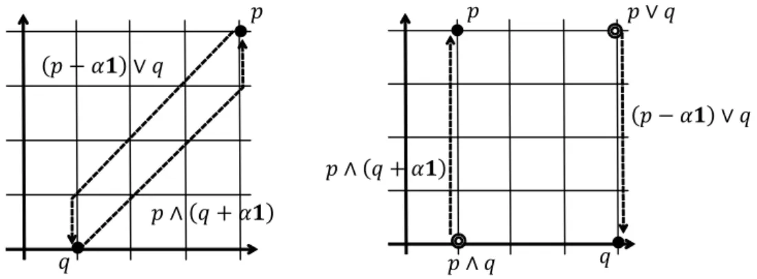
It is known that L♮-convexity is equivalent to the following property (see Figure 1):
[Translation Submodularity]
g(p) + g(q)≥ g((p − α1) ∨ q) + g(p ∧ (q + α1)) (∀p, q ∈ dom g, ∀α ∈ Z+). (2.4)
L♮-convexity is also equivalent to a discrete version of mid-point convexity:
[Discrete Mid-point Convexity]
g(p) + g(q) ≥ g (⌈ p + q 2 ⌉) + g (⌊ p + q 2 ⌋) (∀p, q ∈ dom g), (2.5) where ⌈p+q2 ⌉ and ⌊p+q2 ⌋ denote the integral vectors obtained by component-wise rounding up and rounding down of the vector p+q2 , respectively.
From the discussion above, we obtain the following equivalence.
Theorem 2.1 ([15]). For a function g :Zn→ R ∪ {+∞} the following three properties are
equivalent:
(a) L♮-convexity, i.e., L-convexity of ˜g in (2.3),
(b) translation submodularity (2.4), (c) discrete mid-point convexity (2.5).
Figure 1: Vectors (p− α1) ∨ q and p ∧ (q + α1) in the translation submodularity (2.4): (Left) Case of p≥ q, (Right) Case of p(1) > q(1) and p(2) < q(2). Trajectories of the two vectors when α is increased from 0 is drawn by dashed arrows. Note that if p ≤ q, then (p− α1) ∨ q = q and p ∧ (q + α1) = p for every α ≥ 0.
By its definition, the concept of L♮-convex function is essentially equivalent to the concept
of L-convex function. On the other hand, L-convex function can be seen as a special case of L♮-convex function. Indeed, translation submodularity of an L-convex function can be
shown as follows, where p, q∈ dom g and α ∈ Z+:
g(p) + g(q) = g(p− α1) + αr + g(q) (by (2.2))
≥ g((p − α1) ∨ q) + g((p − α1) ∧ q) + αr (by (2.1)) = g((p− α1) ∨ q) + g(p ∧ (q + α1)) (by (2.2)).
2.2. Examples
We present several examples of L-convex and L♮-convex functions. See Section 3.3 for more examples.
Example 2.2 (linear functions). For a real vector c ∈ Rn, the linear function given by
g(p) = ∑ni=1c(i)p(i) (p ∈ Zn) is L-convex as well as L♮-convex. Moreover, given a(i, j) ∈
Z ∪ {−∞} (i, j ∈ N, i ≤ j) and b(i, j) ∈ Z ∪ {+∞} (i, j ∈ N, i ≤ j), the function g :Zn→ R ∪ {+∞} given by
dom g ={p ∈ Zn| a(i, i) ≤ p(i) ≤ b(i, i) (i ∈ N),
a(i, j)≤ p(i) − p(j) ≤ b(i, j) (i, j ∈ N, i < j)}, g(p) =
n
∑
i=1
c(i)p(i) (p∈ dom g)
is L♮-convex, provided that dom g is nonempty; the function g is L-convex if a(i, i) =−∞
(i∈ N) and b(i, i) = +∞ (i ∈ N), in addition.
Example 2.3 (quadratic functions). A quadratic function g(p) = p⊤Ap (p∈ Zn) given by
an n× n real symmetric matrix A is L♮-convex if and only if each off-diagonal component a(i, j) (i, j ∈ N, i ̸= j) is non-positive and the sum of components in each row (or column) ∑n
j=1a(i, j) (i∈ N) is non-negative [41].
Example 2.4 (maximum-value functions). Define
g(p) = max{p(1), p(2), . . . , p(n)} (p∈ Zn), g0(p) = max{0, p(1), p(2), . . . , p(n)} (p∈ Zn).
Then, g is an L-convex function and g0 is an L♮-convex function. We also consider the
following functions associated with real numbers a(0), a(1), . . . , a(n), b(0), b(1), . . . , b(n)∈ R: ˜
g(p) = max
1≤i≤n{p(i) + a(i)} − min1≤i≤n{p(i) + b(i)} (p∈ Z n),
˜
g0(p) = max
0≤i≤n{p(i) + a(i)} − min0≤i≤n{p(i) + b(i)} (p∈ Z n),
where p(0) = 0. Function ˜g is L-convex and ˜g0 is L♮-convex [37]. 2.3. Properties of minimizers
Minimizers of L-convex and L♮-convex functions enjoy various properties. Since an L♮-convex function satisfies submodularity (see (2.4)), the set of minimizers forms a sublattice of Zn.
We denote by arg min g the set of minimizers of a function g :Zn→ R ∪ {+∞}, i.e.,
arg min g ={p ∈ Zn| g(p) ≤ g(q) (∀q ∈ Zn)}.
Theorem 2.5. Let g :Zn → R ∪ {+∞} be an L♮-convex function. (i) For p, q ∈ arg min g, we have p ∨ q, p ∧ q ∈ arg min g.
(ii) Minimal and maximal minimizers of g are uniquely determined if they exist. In par-ticular, if arg min g is bounded, then minimal and maximal minimizers of g are uniquely determined.
It should be noted that there may exist many minimal and maximal minimizers for a general function.
The global minimality of an L♮-convex function can be characterized by the local min-imality with respect to a certain neighborhood. For a function g : Zn → R ∪ {+∞},
p ∈ dom g, and d ∈ Zn, we denote by g′(p; d) the slope of g at p in the direction d, i.e.,
g′(p; d) = g(p + d)− g(p).
Theorem 2.6 ([31–33]). Let g :Zn→ R ∪ {+∞} be an L♮-convex function and p∈ dom g. Then, we have p ∈ arg min g if and only if g′(p; d) ≥ 0 holds for every d ∈ {0, +1}n∪
{0, −1}n.
For p ∈ dom g, a vector d = d∗ ∈ {0, +1}n ∪ {0, −1}n minimizing g′(p; d) is called a steepest descent direction of g at p. Since g′(p; 0) = 0, every steepest descent direction d∗ satisfies g′(p; d∗)≤ g′(p; 0) = 0. Therefore, we have the following equivalence:
g′(p; d)≥ 0 (∀d ∈ {0, +1}n∪ {0, −1}n) ⇐⇒ g′(p; d
∗) = 0 (∀d∗ : steepest descent direction at p)
⇐⇒ d∗ = 0 is a steepest descent direction at p.
Due to L♮-convexity, minimal and maximal steepest descent directions are uniquely
deter-mined.
If we know in advance that a vector p ∈ dom g is a lower bound (or an upper bound) of some minimizer, then we can characterize the global minimality of p by using the local minimality with respect to a smaller neighborhood.
Theorem 2.7 (cf. [44]). Let g :Zn→ R ∪ {+∞} be an L♮-convex function, and p∈ dom g be a vector that is a lower bound of some minimizer p∗ of g (i.e., p≤ p∗ holds).
(i) There exists a steepest descent direction d of g at p such that d≥ 0 (i.e., d ∈ {0, +1}n).
(ii) p∈ arg min g holds if and only if g′(p; d)≥ 0 holds for every d ∈ {0, +1}n.
Theorem 2.8 (cf. [44]). Let g :Zn→ R ∪ {+∞} be an L♮-convex function, and p∈ dom g be a vector that is an upper bound of some minimizer p∗ of g (i.e., p≥ p∗ holds).
(i) There exists a steepest descent direction d of g at p such that d≤ 0 (i.e., d ∈ {0, −1}n).
For an L-convex function g that has a minimizer p∗, the real number r in the condition (2.2) must be equal to zero, from which follows that p∗ + α1 is also a minimizer of g for every α∈ Z. Therefore, every p ∈ dom g is a lower bound of some minimizer as well as an upper bound of another minimizer, which, together with Theorems 2.7 and 2.8, implies the following property.
Theorem 2.9. For an L-convex function g :Zn→ R ∪ {+∞} and a vector p ∈ dom g, the
following three conditions are equivalent:
(a) p∈ arg min g, (b) g′(p; d) ≥ 0 (∀d ∈ {0, +1}n), (c) g′(p; d)≥ 0 (∀d ∈ {0, −1}n). 3. Minimization Algorithms
Minimization algorithms for L-convex and L♮-convex functions are presented in this section.
Since the minimization of an L-convex function is a special case of the minimization of an L♮-convex function, we mainly deal with the latter. Throughout this section, we assume
that g :Zn→ R ∪ {+∞} is an L♮-convex function with bounded dom g. 3.1. Fundamental algorithms
The first algorithm finds a minimizer by iteratively moving a solution along steepest descent directions.
Algorithm 1 (Greedy).
Step 0: Select an initial solution p0 ∈ dom g arbitrarily, and set p := p0.
Step 1: If g′(p; d) ≥ 0 holds for every d ∈ {0, +1}n∪ {0, −1}n, then output p and stop. Step 2: Find d = d∗ ∈ {0, +1}n∪ {0, −1}n minimizing g′(p; d). Set p := p + d
∗ and
go to Step 1.
By Theorem 2.6, the algorithm Greedy outputs a minimizer of an L♮-convex function
when it terminates. Since the function value g(p) decreases strictly in each iteration and dom g is bounded, the algorithm Greedy terminates in a finite number of iterations. Note that the computation of a steepest descent direction in each iteration can be done in poly-nomial time (in n) by reduction to the minimization of submodular set functions ρ+
p, ρ−p
given by
ρ+p(X) = g′(p; +eX), ρ−p(X) = g′(p;−eX) (X ⊆ N),
where eX ∈ {0, +1}ndenotes the characteristic vector of X ⊆ N; see [25, 49] for the
strongly-polynomial time algorithms for submodular set function minimization.
If a lower bound of a minimizer of g is available as the initial solution, then an increasing-type steepest descent algorithm can be applied by Theorem 2.7. Here, an “increasing-type” algorithm means that in the algorithm each component of vector p is monotonically increasing (non-decreasing).
Algorithm 2 (GreedyUp).
Step 0: Select an initial solution p0 ∈ dom g that is a lower bound of some minimizer of g,
and set p := p0.
Step 1: If g′(p; d) ≥ 0 holds for every d ∈ {0, +1}n, then output p and stop.
Step 2: Find d = d∗ ∈ {0, +1}n minimizing g′(p; d). Set p := p + d∗ and go to Step 1. Similarly, if an upper bound of some minimizer of g is available as the initial solution, then a decreasing-type steepest descent algorithm can be applied by Theorem 2.8.
Algorithm 3 (GreedyDown).
Step 0: Select an initial solution p0 ∈ dom g that is an upper bound of some minimizer of g,
and set p := p0.
Step 1: If g′(p; d) ≥ 0 holds for every d ∈ {0, −1}n, then output p and stop.
ϭ ϭ ϭ Ϯ ϯ Ϭ Ϭ Ϭ Ϭ ϭ ϭ Ϭ Ϭ Ϭ ϭ Ϯ ϭ ϭ ϭ ϭ ϯ Ϯ Ϯ Ϯ Ϯ K
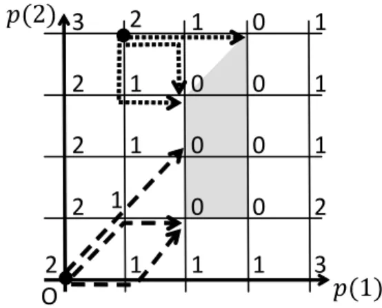
Figure 2: The behavior of the steepest descent algorithms. Each number associated with each integer lattice point denotes the function value of g at the point. The shaded region shows the set of minimizers of g.
Remark 3.1. The algorithm GreedyUp is originally proposed as a minimization algorithm
of L-convex functions (see, e.g., [33, Section 10.3.1]). If an L-convex function g has a minimizer, then for every initial vector p0 ∈ dom g there exists some minimizer p∗ of g
such that p∗ ≥ p0 (see the discussion just before Theorem 2.9). Hence, a minimizer of
L-convex function g can be obtained by GreedyUp with an arbitrarily chosen initial vector p0. Similarly, GreedyDown can also be applied to an L-convex function.
Remark 3.2. The behavior of vector p in the algorithm Greedy applied to an L♮-convex function g :Zn→ R ∪ {+∞} coincides with the behavior of the original variable vector p in
GreedyUp applied to L-convex function ˜g :Zn+1 → R ∪ {+∞} with n + 1 variables given by (2.3).
3.2. A numerical example
To illustrate the behavior of the steepest descent algorithms explained above, we consider a numerical example of L♮-convex function g :Z2 → R∪{+∞} given as follows (see Figure 2):
dom g ={(p(1), p(2)) ∈ Z2 | 0 ≤ p(i) ≤ 4 (i = 1, 2)}, g(p(1), p(2)) = max(0, −p(1) + 2, −p(2) + 1, p(1) − 3,
−p(1) + p(2) − 1, 2p(1) − p(2) − 5) ((p(1), p(2))∈ dom g). L♮-convexity of this function can be checked by using the translation submodularity (2.4)
or discrete-midpoint convexity (2.5) (see Theorem 2.1).
Suppose that the algorithm Greedy is applied to the function g with the initial solution p0 = (1, 4). Then, the trajectory of vector p is given by one of the three dotted arrows in
Figure 2 starting from (1, 4). In particular, the minimizer found by the algorithm is either of (3, 4) and (2, 3).
We then suppose that the algorithm Greedy or GreedyUp is applied to g with another initial solution p0 = (0, 0). Then, the trajectory of vector p is given by one of the three
dashed arrows in Figure 2 starting from (0, 0). In particular, the minimizer found by the algorithm is either of (2, 1) and (2, 2).
3.3. Steepest descent algorithms in other research fields
We show that various optimization algorithms proposed independently in other research fields can be seen as steepest descent algorithms in Section 3.1 applied to special L♮-convex
3.3.1. Hassin’s algorithm for the minimum cost flow problem
Given a directed graph G = (V, E), non-negative edge capacity c(e)∈ R+(e∈ E), and edge
cost γ(e)∈ R (e ∈ E), the minimum cost flow problem (minimum cost circulation problem) is formulated as follows: Minimize ∑ (u,v)∈E γ(u, v)x(u, v) subject to ∑ v:(u,v)∈E x(u, v)− ∑ v:(v,u)∈E x(v, u) = 0 (u∈ V ), 0≤ x(u, v) ≤ c(u, v) ((u, v) ∈ E).
This is a linear programming problem, and its dual is given as Maximize gH(p) ≡
∑
(u,v)∈E
c(u, v) min{0, p(u) − p(v) + γ(u, v)} subject to p(v)∈ R (v ∈ V ).
Hassin’s algorithm [21] solves the minimum cost flow problem by finding an optimal solution of the dual problem, instead of solving the primal problem directly.
Assume that edge cost γ(u, v) is integer for each (u, v)∈ E. Then, it can be shown that the dual problem has an integral optimal solution. Hence, we may restrict the values of dual variables p(v) (v ∈ V ) to integers, and the objective function gH can be regarded as
a function in discrete variables. It is known that this function gH is an L-concave function
in discrete variables (see [32, 33, 36, 42]). Moreover, Hassin’s algorithm coincides with the algorithm GreedyUp (more precisely, the algorithm GreedyUpMinimal in Section 3.4) applied to L-convex function −gH (see [43] for details).
For the minimum cost submodular flow problem, which is a generalization of the min-imum cost flow problem, Chung–Tcha [7] proposed an algorithm by generalizing Hassin’s algorithm under the integrality assumption for the problem input. This algorithm can also be seen as a (variant of) the algorithm GreedyUp applied to an L-convex function arising from the dual of the minimum cost submodular flow problem (see [43] for details).
3.3.2. Discrete optimization approach in computer vision
Given an undirected graph G = (V, E) and univariate convex functions φv :Z → R ∪ {+∞}
(v ∈ V ), ψuv :Z → R ∪ {+∞} ((u, v) ∈ E), consider the following optimization problem:
(P): Minimize gCV(p) ≡ ∑ v∈V φv(p(v)) + ∑ (u,v)∈E ψuv(p(v)− p(u)) subject to p(v)∈ Z (v ∈ V ).
Here, we say that a univariate function φ :Z → R ∪ {+∞} is convex if 2φ(α) ≤ φ(α − 1) + φ(α + 1) holds for every α∈ Z with φ(α) < +∞. The objective function gCV of the problem
(P) is an L♮-convex function. Moreover, if the first term∑
v∈V φv(p(v)) is removed from the
function gCV, then the resulting function is an L-convex function (see [32, 33, 36, 42]).
The problem (P) is used to process various tasks in computer vision such as panoramic image stitching [54], image restoration [6], minimization of total variation [9], phase unwrap-ping in SAR images [4], etc. In these problems, the vertex set V of the graph G corresponds to the set of pixels in a given image, and edges of the graph represent the neighborhood relation of pixels. Variable p(v) represents the label of the pixel v such as disparity, inten-sity, etc. The function φv for each v ∈ V is called the data term and used to evaluate the
label of the pixel v. The function ψuv for (u, v)∈ E is called the smoothness term and used
to evaluate the difference of the labels for a pair of adjacent pixels u and v. The objective function gCV of the problem (P) is called an energy function in the context of Markov
ran-dom field [18], and its minimizer corresponds to a set of labels maximizing the a-posteriori probability.
In computer vision, many algorithms for the problem (P) have been proposed (see, e.g., [4, 27]). In particular, Kolmogorov [27] proposed a general framework of minimization algo-rithms that includes the algoalgo-rithms Greedy, GreedyUp, and GreedyDown as special cases. An algorithm by Bioucas-Dias–Valad˜ao [4] coincides with the algorithm GreedyUp applied to the problem (P) without the first term ∑v∈V φv(p(v)).
3.3.3. Iterative auction in auction theory
Consider an auction with multiple indivisible items. In such an auction, the auctioneer needs to find “appropriate” prices of items as well as an “appropriate” allocation of items to bidders. An ascending auction due to Ausubel [3], which is an algorithm for computing such “appropriate” prices by using the Lyapunov function, can be regarded as an application of the algorithm GreedyUp to a special L♮-convex function. We discuss this topic in more
details in Section 6.
3.4. Computation of minimal and maximal minimizers
For an L♮-convex function with bounded effective domain, minimal and maximal minimizers
are uniquely determined by Theorem 2.5. We show that unique minimal and maximal minimizers can be computed by using variants of the algorithms in Section 3.1.
We first consider the minimal minimizer. The minimal minimizer of function g is the same as the unique minimizer of the function
gε(p) = g(p) + ε n
∑
i=1
p(i),
where ε is a sufficiently small positive number. Since the function gε is also an L♮-convex
function, its minimizer can be computed by the algorithm GreedyUp, although we need to select the value of ε appropriately so that a minimizer of gε is also a minimizer of
g. In fact, we do not need to compute such ε explicitly. The behavior of the algorithm GreedyUp applied to the function gε with a sufficiently small ε > 0 coincides with the
behavior of GreedyUpMinimal to be explained below applied to the original function g. The difference between GreedyUpMinimal and GreedyUp is in the choices of the initial solution and a steepest descent direction in each iteration.
Algorithm 4 (GreedyUpMinimal).
Step 0: Select an initial solution p0 ∈ dom g that is a lower bound of the minimal minimizer
of g, and set p := p0.
Step 1: If g′(p; d) ≥ 0 holds for every d ∈ {0, +1}n, then output p and stop. Step 2: Find a (unique) minimal minimizer d = d∗ ∈ {0, +1}n of g′(p; d).
Set p := p + d∗ and go to Step 1.
Note that a minimal minimizer d = d∗ ∈ {0, +1}n of g′(p; d) found in Step 2 is uniquely
determined due to the submodularity of g.
Proposition 3.3. For an L♮-convex function g :Zn→ R ∪ {+∞} with bounded dom g, the algorithm GreedyUpMinimal outputs the unique minimal minimizer.
Based on a similar idea, the algorithm Greedy can also be used to find the minimal minimizer by modifying the condition of the termination and the choice of a steepest descent direction.
Algorithm 5 (GreedyMinimal).
Step 0: Select an initial solution p0 ∈ dom g arbitrarily and set p := p0.
Step 1: Find a (unique) minimal minimizer d = d∗ ∈ {0, +1}n∪ {0, −1}n of g′(p; d).
Step 2: If d∗ = 0, then output p and stop. Otherwise, set p := p + d∗ and go to Step 1.
Proposition 3.4. For an L♮-convex function g :Zn→ R ∪ {+∞} with bounded dom g, the algorithm GreedyMinimal outputs the unique minimal minimizer.
By modifying the algorithm GreedyDown in a similar way, we can obtain the algorithm GreedyDownMinimal that finds the minimal minimizer.
Remark 3.5. Iteration of the algorithm GreedyMinimal does not necessarily stop even if
the current vector p is a minimizer of g. For example, let us consider the L♮-convex function
g in Section 3.2. If we apply GreedyMinimal with the initial solution p0 = (1, 4), then
the trajectory of p is given as (1, 4)→ (1, 3) → (2, 3) → (2, 2) → (2, 1), which reaches the minimal minimizer (2, 1) after passing through the minimizers (2, 3) and (2, 2).
We then consider the computation of the maximal minimizer. For a general function g : Zn → R ∪ {+∞}, a vector p is a maximal minimizer of g if and only if −p is a
minimal minimizer of the function h :Zn → R ∪ {+∞} defined by h(q) = g(−q) (q ∈ Zn).
Moreover, function g is L♮-convex if and only if function h is L♮-convex. Hence, an algorithm for computing the maximal minimizer of an L♮-convex function can be easily obtained by
modification of an algorithm for the minimal minimizer. For example, we can obtain the following algorithm for the unique maximal minimizer of L♮-convex function g by rewriting the algorithm GreedyUpMinimal applied to L♮-convex function h in terms of the function
g; the resulting algorithm can be seen as a variant of the algorithm GreedyDown.
Algorithm 6 (GreedyDownMaximal).
Step 0: Select an initial solution p0 ∈ dom g that is an upper bound of the maximal minimizer
of g, and set p := p0.
Step 1: If g′(p; d) ≥ 0 holds for every d ∈ {0, −1}n, then output p and stop. Step 2: Find a (unique) maximal minimizer d = d∗ ∈ {0, −1}n of g′(p; d).
Set p := p + d∗ and go to Step 1.
Proposition 3.6. For an L♮-convex function g :Zn→ R ∪ {+∞} with bounded dom g, the algorithm GreedyDownMaximal outputs the unique maximal minimizer.
By using similar ideas, we can obtain algorithms GreedyMaximal and GreedyUp-Maximal for the maximal minimizer as variants of Greedy and GreedyUp.
3.5. Use of long step length
In all the algorithms explained in Sections 3.1 and 3.4, the current vector p repeats moving along a certain direction by unit step length. We consider a modification of the algorithms where the vector p moves along the same steepest descent direction d∗ as far as the value of the slope g′(p; d∗) in the steepest descent direction does not change.
For example, if this modification is applied to the algorithm GreedyUp, the following algorithm is obtained. For a vector p ∈ dom g and a direction d ∈ {0, +1}n∪ {0, −1}n, we define the value ¯c(p; d)∈ Z ∪ {+∞} by
¯
c(p; d) = sup{λ ∈ Z+ | g(p + λd) − g(p) = λ g′(p; d)}. Algorithm 7 (GreedyUp-LS).
Step 0: Select an initial solution p0 ∈ dom g that is a lower bound of some minimizer of g,
and set p := p0.
Step 2: Find d = d∗ ∈ {0, +1}n minimizing g′(p; d). Set λ := ¯c(p; d
∗), p := p + λd∗, and
go to Step 1.
As shown in Section 4.2, this algorithm can be seen as a special implementation of GreedyUp. In particular, the output of GreedyUp-LS is a minimizer of g.
Computation of a steepest descent direction is essentially equivalent to the minimization of a submodular set function (see Section 3.1), for which we require quite large running time to obtain a minimizer (see, e.g., [25, 49]). Therefore, the use of long step length helps to reduce the total running time. Note that the computation of the step length ¯c(p; d∗) can be done by binary search; for the special cases of L♮-convex functions shown in Sections 2.2
and 3.3, the step length can be computed more easily.
Long step length can be used to other steepest descent algorithms in a similar way; we omit the details in this paper.
4. Analysis of Number of Iterations in Steepest Descent Algorithms
We analyze the number of iterations required by the algorithms in Section 3. In Section 4.1, the precise bounds for the steepest descent algorithms and its variants are provided in terms of the distance to minimizers. In Section 4.2, we consider an increasing-type steepest descent algorithm using long step length, and obtain an upper bound of the number of iterations by using the slope of steepest descent directions. While other minimization algorithms can be analyzed in a similar way, we omit the details in this paper.
In the following, let g : Zn → R ∪ {+∞} be an L♮-convex function with bounded dom g.
4.1. Analysis by using the distance to minimizers
We analyze the number of iterations of algorithms by using the distance from the current vector p ∈ Zn to minimizers. In the analysis we use two kinds of distance. We define a
function ˆµ :Zn → Z+∪ {+∞} by
ˆ µ(p) =
{
min{∥p∗− p∥∞| p∗ ∈ arg min g, p∗ ≥ p} (if {p∗ ∈ arg min g | p∗ ≥ p} ̸= ∅),
+∞ (otherwise).
(4.1) That is, ˆµ(p) is the ℓ∞-distance between a vector p and a nearest minimizer p∗ under the condition p∗ ≥ p. We also define a function µ : Zn → Z
+ by
µ(p) = min{∥p∗− p∥+∞+∥p∗− p∥−∞| p∗ ∈ arg min g} (p∈ Zn), (4.2) where
∥p∗− p∥+∞ = maxi∈N max(0, p∗(i)− p(i)),
∥p∗− p∥−∞ = maxi∈N max(0,−p∗(i) + p(i)).
Function µ(p) gives a distance between p and a nearest minimizer p∗.
Due to the L♮-convexity of g, the functions µ(p) and ˆµ(p) have the following relationship;
the proof is given in Appendix.
Proposition 4.1 (K. Murota). ˆµ(p) = µ(p) holds for a vector p ∈ Zn such that {q ∈ arg min g | q ≥ p} ̸= ∅.
Example 4.2. Consider the example of an L♮-convex function in Section 3.2 (see Figure 2).
We have ˆµ(p) = µ(p) = 2 for p = (1, 4). The value ˆµ(p) = 2 is attained by the minimizer (3, 4), while µ(p) = 2 is attained by both of the two minimizers (3, 4) and (2, 3).
We first analyze the two increasing-type steepest descent algorithms, GreedyUp and GreedyUpMinimal. Suppose that a vector p ∈ dom g is a lower bound of some minimizer of function g. We consider the unique minimal minimizer p∗ of g under the condition p∗ ≥ p, which we denote by ˆp. Recall that in an increasing-type algorithm each component of vector p increases monotonically. Desirable properties of increasing-type algorithms (for an unknown ˆp) are as follows:
(a) for each i∈ arg maxj∈N{ˆp(j)−p(j)}, the value of p(i) is increased if maxj∈N{ˆp(j)−
p(j)} > 0.
(b) for each i∈ N with ˆp(i) − p(i) = 0, the value of p(i) is unchanged.
The next proposition shows that if vector p is updated by using a steepest descent direction d ∈ {0, +1}n, then (a) holds; moreover, (b) also holds if d is the minimal steepest descent direction, in particular. We denote supp+(d) ={i ∈ N | d(i) > 0} for d ∈ Zn.
Proposition 4.3 ([44]). Let p∈ dom g be a vector that is a lower bound of some minimizer
of g, and ˆp∈ arg min g be a (unique) minimal minimizer of g under the condition ˆp ≥ p. (i) For every steepest descent direction d∈ {0, +1}nat p, we have arg max
j∈N{ˆp(j)−p(j)} ⊆
supp+(d). In addition, p∗ = ˆp∨(p+d) is a (unique) minimal minimizer under the condition p∗ ≥ p + d and satisfies ∥p∗− (p + d)∥∞=∥ˆp − p∥∞− 1.
(ii) For the (unique) minimal steepest descent direction d∈ {0, +1}n at p, we have
supp+(d)∩ {i ∈ N | ˆp(i) = p(i)} = ∅, ˆp ≥ p + d, ∥ˆp − (p + d)∥∞ =∥ˆp − p∥∞− 1.
From the proposition above, the precise bounds for the number of updates of p in GreedyUp and in GreedyUpMinimal can be obtained. In general, if we update vector p by increasing each component at most one, then the value ˆµ(p) decreases by at most one. Hence, ˆµ(p0) gives a lower bound for the number of iterations required by any
increasing-type algorithm with the initial solution p0. In fact, it is shown that the number of updates
of p in GreedyUp is exactly equal to ˆµ(p0). We define
Φg = max{∥p − q∥∞| p, q ∈ dom g},
which gives the “size” of the effective domain of g.
Theorem 4.4 (cf. [44]).
(i) If vector p is updated in an iteration of the algorithm GreedyUp, then the value ˆµ(p) decreases by one.
(ii) The number of update of vector p in GreedyUp is equal to ˆµ(p0) and at most Φg.
(iii) The minimizer p∗ ∈ arg min g found by GreedyUp satisfies ∥p∗− p0∥∞ = ˆµ(p0).
This theorem implies that the trajectory of vector p generated by GreedyUp is a shortest path (with respect to ℓ∞-distance) from the initial solution p0 to a nearest minimizer
p∗ under the condition p∗ ≥ p0.
Corollary 4.5 ([44, 46]). The algorithm GreedyUpMinimal outputs the unique minimal
minimizer p
∗ after vector p is updated ∥p∗− p0∥∞ times.
Example 4.6. We consider the example for the behavior of the algorithm in Section 3.2.
If we apply the algorithm GreedyUp with the initial solution p0 = (0, 0), then the output
of the algorithm is either p∗ = (2, 1) or p∗ = (2, 2), each of which is a nearest minimizer to p0 (i.e., a minimizer with the minimum value of ∥p∗ − p0∥∞) under the condition p∗ ≥ p0.
The number of updates of p in the algorithm is equal to ˆµ(p0) = 2, the distance from
p0 to a nearest minimizer. Three possible trajectories of p in the algorithm GreedyUp
solution p0 = (0, 0) to a nearest minimizer. Also, if we apply GreedyUpMinimal, then
the trajectory of p is given as (0, 0) → (1, 0) → (2, 1), and its output p∗ = (2, 1) is the minimal minimizer.
A similar result can be obtained for the decreasing-type steepest descent algorithms GreedyDown and GreedyDownMaximal. For a vector p ∈ dom g that is an upper bound of some minimizer of L♮-convex function g, we define the value ˇµ(p)∈ Z
+ by
ˇ µ(p) =
{
min{∥p∗− p∥∞| p∗ ∈ arg min g, p∗ ≤ p} (if {p∗ ∈ arg min g | p∗ ≤ p} ̸= ∅),
+∞ (otherwise).
Proposition 4.7 (K. Murota). ˇµ(p) = µ(p) holds for a vector p ∈ Zn such that {q ∈ arg min g | q ≤ p} ̸= ∅.
Theorem 4.8 (cf. [44]).
(i) If vector p is updated in an iteration of the algorithm GreedyDown, then the value ˇ
µ(p) decreases by one.
(ii) The number of update of vector p in GreedyDown is equal to ˇµ(p0) and at most Φg.
(iii) The minimizer p∗ ∈ arg min g found by GreedyDown satisfies ∥p∗−p0∥∞= ˇµ(p0). Corollary 4.9 ([44, 46]). The algorithm GreedyDownMaximal outputs the unique
max-imal minimizer p∗ after vector p is updated ∥p∗− p0∥∞ times.
Remark 4.10. We consider the special case where g : Zn → R ∪ {+∞} is an L-convex
function. If g has a minimizer, then for every vector p0, there exists a minimizer p∗ satisfying
p∗ ≥ p0 and mini∈N{p∗(i)− p0(i)} = 0 (see the discussion just before Theorem 2.9). Hence,
ˆ
µ(p0)≤ Ψg holds with
Ψg = max{∥p − q∥∞ | p, q ∈ dom g, min
i∈N{p(i) − q(i)} = 0}.
If the value Ψg is finite, then the increasing-type steepest descent algorithms GreedyUp
and GreedyUpMinimal terminate in at most Ψg iterations. Similarly, the decreasing-type
steepest descent algorithms GreedyDown and GreedyDownMaximal terminate in at most Ψg iterations.
By generalizing the analysis used in Theorem 4.4, we can obtain the exact bound for the number of updates of p in the algorithms Greedy and GreedyMinimal.
Theorem 4.11 ([44]).
(i) If vector p is updated in an iteration of the algorithm Greedy, then the value µ(p) decreases by one.
(ii) The number of update of vector p in Greedy is equal to µ(p0) and at most 2Φg.
(iii) The minimizer p∗ ∈ arg min g found by Greedy satisfies ∥p∗− p0∥+∞+∥p∗− p0∥−∞ =
µ(p0).
It follows from this theorem that the trajectory of vector p generated by the algorithm Greedy is a shortest path (with respect to a certain distance) from the initial solution p0
to a nearest minimizer p∗.
Corollary 4.12 ([44]). The algorithm GreedyMinimal outputs the unique minimal
min-imizer p
∗ after vector p is updated ∥p∗− p0∥+∞+∥p∗− p0∥−∞ times.
Example 4.13. We reconsider Example 3.2. When we apply the algorithm Greedy with
the initial solution p0 = (1, 4), the output of the algorithm is either of p∗ = (3, 4) and
p∗ = (2, 3), both of which are nearest minimizers to p0 (with respect to the distance ∥p∗−
p∥+
∞+∥p∗− p∥−∞), and the number of updates of p is equal to µ(p0) = 2, the distance to
by dotted arrows in Figure 2, each of which is a shortest path from the initial solution p0 = (1, 4) to a nearest minimizer.
Remark 4.14. As upper bounds for the number of updates of a vector in the algorithm
Greedy, 2nΦg is shown by Murota [34] and 2Φg by Kolmogorov–Shioura [28]. The result
presented in this section (Theorem 4.11) is a refinement of these results by Murota–Shioura [44].
Remark 4.15. Recently, Hirai [22, 23] introduced the concept of L-convex function on
oriented modular graphs, as a generalization of L♮-convex function on integer lattice points. In this concept, a function is defined on the set of vertices, and the neighborhood of each vertex is defined by using oriented edges. In this framework, an L♮-convex function on integer
lattice points can be regarded as an L-convex function on a grid graph with an appropriate edge orientation. Hirai [22, 23] proposed a steepest descent algorithm for minimization of an L-convex function on an oriented modular graph, and showed that the number of iterations is equal to a certain distance between the initial solution and the minimizer output by the algorithm. This result is closely related to Theorems 4.4 and 4.11 presented in this section.
4.2. Analysis by the slope of steepest descent direction
We consider a variant of the algorithm GreedyUpMinimal using long step length, which we denote GreedyUpMinimal-LS. In this section, we analyze the number of iterations required by GreedyUpMinimal-LS by using slopes of steepest descent directions. For this, we first show a property concerning the slope of a steepest descent direction in each iteration of GreedyUpMinimal (i.e., the algorithm using the unit step length) and clarify the relationship between GreedyUpMinimal and GreedyUpMinimal-LS.
We show that in GreedyUpMinimal, the absolute value |g′(p; d)| of the slope of a steepest descent direction d is non-increasing; moreover, if the unique minimal steepest descent direction is used, then the absolute value|g′(p; d)| of the slope decreases strictly or the set supp+(d) of non-zero components in a steepest descent direction d monotonically
increases (in the sense of set inclusion). Note that g′(p; d) ≤ 0 holds for every p ∈ dom g and every steepest descent direction d at p.
Proposition 4.16 (cf. [16]). Let p∈ dom g, and d ∈ {0, +1}nbe a steepest descent direction
at p, and ed∈ {0, +1}n be a steepest descent direction at p + d. (i) 0≥ g′(p + d; ed)≥ g′(p; d) holds.
(ii) Suppose that d and ˜d are minimal steepest descent directions at p and p + d, respectively. Then, at least one of the following two conditions holds:
(a) g′(p + d; ed) > g′(p; d), (b) g′(p + d; ed) = g′(p; d) and supp+( ed)⊇ supp+(d). For p∈ dom g, let d ∈ {0, +1}nbe a steepest descent direction at p. Proposition 4.16 (i)
implies that d is also a steepest descent direction at p + λd for every λ∈ Z+ with 0≤ λ <
¯
c(p; d). Hence, the algorithm GreedyUpMinimal-LS using long step lengths can be re-garded as a variant of the algorithm GreedyUpMinimal, where the same steepest descent direction as in the previous iteration is used whenever possible. From this observation follows that the trajectory of vector p of the algorithm GreedyUpMinimal-LS is the same as the trajectory of vector p of GreedyUpMinimal, and the output of GreedyUpMinimal-LS is a minimizer of function g.
An upper bound for the number of iterations of GreedyUpMinimal-LS can be ob-tained by using Proposition 4.16 (ii). When vector p is updated to ˜p = p + λd with λ = ¯c(p; d), the slopes g′(p; d) and g′(˜p; d) satisfy 0 ≥ g′(˜p; d) > g′(p; d) by the definition of
λ and the discrete mid-point convexity (2.5) of g. Therefore, Proposition 4.16 (ii) implies that for the unique minimal steepest descent direction ed ∈ {0, +1}n at ˜p, at least one of g′(˜p; ed) > g′(p; d) and supp+( ed)⊋ supp+(d) holds if g′(p; d) < 0. Since the slope of a
steep-est descent direction is equal to zero at the termination of the algorithm, the next theorem follows.
Theorem 4.17. For an integer-valued L♮-convex function g, the number of iterations of the
algorithm GreedyUpMinimal-LS is at most n · max{−g′(p0; d)| d ∈ {0, +1}n}.
Remark 4.18. Consider the example of the minimum cost flow problem in Section 3.3.1.
The function gH is integer-valued if cost c(u, v) and capacity γ(u, v) are integer-valued for
every edge (u, v)∈ E. Hence, from Theorem 4.17 the following upper bound for the number of iterations of Hassin’s algorithm can be obtained:
n· max{gH′ (p0; d)| d ∈ {0, +1}n}.
Recall that function−gH is an L♮-convex function and its slope is given by −g′H(p; d). This
bound coincides with the one shown in Hassin [21, Corollary 3]. Since the slope gH′ (p; d) at a vector p∈ dom gH can be represented as
g′H(p; d) = ∑
(u,v)∈E′
c(u, v)− ∑
(u,v)∈E′′
c(u, v)
for some subsets E′, E′′⊆ E of edges, we have g′H(p0; d)≤
∑
(u,v)∈E
|c(u, v)|.
From this we obtain an upper bound n·∑(u,v)∈E|c(u, v)| for the number of iterations of Hassin’s algorithm, which is independent of the choice of the initial solution p0.
5. Minimization of L-convex Function in Continuous Variables
The concepts of L-convexity and L♮-convexity naturally extend to functions in continuous
variables. Moreover, the minimization algorithms shown in Section 3 as well as their prop-erties can also be extended to L-convex and L♮-convex functions in continuous variables. 5.1. Definition of L-convex function in continuous variables
A convex function g :Rn → R∪{+∞} in continuous variables is called an L-convex function [39, 40] if it satisfies the following two properties, where domRg ={p ∈ Rn | g(p) < +∞}:
[Submodularity] g(p) + g(q)≥ g(p ∨ q) + g(p ∧ q) (∀p, q ∈ domRg),
[Linearity in Direction of 1]
∃r ∈ R : g(p + α1) = g(p) + αr (∀p ∈ Rn, ∀α ∈ R).
For an L-convex function g :Rn→ R ∪ {+∞}, the function ˇg : Rn−1 → R ∪ {+∞} with
n− 1 variables given as ˇ
g(q(1), . . . , q(n− 1)) = g(q(1), . . . , q(n − 1), 0)
is called an L♮-convex function [39, 40]. In other words, a convex function g :Rn→ R∪{+∞} is said to be L♮-convex if the function ˜g :Rn+1 → R ∪ {+∞} with n + 1 variables given by
˜
is an L-convex function. As in the case of functions in discrete variables, the function ˜g defined above satisfies the linearity in the direction of 1. Hence, L-convexity of function ˜g is equivalent to submodularity of function ˜g. This means that L♮-convexity of function g is
equivalent to submodularity of function ˜g.
As in the case of functions in discrete variables, L♮-convexity of function g : Rn →
R ∪ {+∞} can be characterized by the translation submodularity:
[Translation Submodularity]
g(p) + g(q)≥ g((p − α1) ∨ q) + g(p ∧ (q + α1)) (∀p, q ∈ domRg, ∀α ∈ R+). Remark 5.1. It should be noted that L♮-convexity cannot be obtained from the mid-point convexity g(p) + g(q)≥ 2g ( p + q 2 ) (∀p, q ∈ domRg).
Under the continuity of a function, the mid-point convexity is equivalent to convexity in the ordinary sense, which is more general than L♮-convexity.
It is clear from their definitions that L-convex and L♮-convex functions in continuous
variables have close relationship with L-convex and L♮-convex functions in discrete variables. If a function g : Rn → R ∪ {+∞} is an L-convex (resp., L♮-convex) function in continuous
variables, then its restriction gZ : Zn → R ∪ {+∞} on integer lattice points is an
L-convex (resp., L♮-convex) function in discrete variables. On the other hand, in the examples of L-convex (resp., L♮-convex) functions in discrete variables shown in Section 2.2, if we
replace the domain Zn with Rn, then we can obtain L-convex (resp., L♮-convex) functions
in continuous variables. In this way, when we are given L-convex and L♮-convex functions in discrete variables, it is often possible to obtain L-convex and L♮-convex functions in
continuous variables by replacing the domain Zn with Rn. Furthermore, it is known that
every L-convex (resp., L♮-convex) function in discrete variables can be extended to an L-convex (resp., L♮-convex) functions in continuous variables (see, e.g., [32, 33, 36, 42]). 5.2. Minimization algorithms and their properties
Minimization algorithms for L♮-convex functions in discrete variables can be naturally
ex-tended to polyhedral L♮-convex functions. A convex function g : Rn → R ∪ {+∞} is said
to be polyhedral if its epigraph {(p, β) | p ∈ Rn, β ∈ R, g(p) ≤ β} is a polyhedron (i.e., represented as the intersection of a finite number of closed half-spaces). In this section, we assume that g :Rn→ R ∪ {+∞} is a polyhedral L♮-convex function.
For p ∈ domRg and d ∈ Rn, the directional derivative g′(p; d) of function g at p in the
direction d is given as
g′(p; d) = lim
λ↓0
g(p + λd)− g(p)
λ .
Since g is a polyhedral convex function, the limit in the right-hand side exists if we allow to have g′(p; d) = +∞.
By its definition, an L♮-convex function g in continuous variables is a convex function
in the ordinary sense. Hence, a vector p∈ domRg is a minimizer if and only if g′(p; d)≥ 0 holds for every direction d∈ Rn. In fact, by L♮-convexity we may restrict our attention only to a finite number of directions to check the minimality of a vector.
Theorem 5.2 ([32, 33, 39]). Let g : Rn → R ∪ {+∞} be a polyhedral L♮-convex function.
Then, a vector p ∈ domRg is a minimizer of g if and only if g′(p; d) ≥ 0 holds for every d∈ {0, +1}n∪ {0, −1}n.
This is an extension of Theorem 2.6 for L♮-convex functions in discrete variables. By
Theorem 5.2, the steepest descent algorithm Greedy-LS using (long) step length in Sec-tion 3 can be naturally extended to a polyhedral L♮-convex function g. For p∈ dom
Rg and
d∈ Rn with g′(p; d) < +∞, we define the value ¯c(p; d) ∈ R ∪ {+∞} by
¯
c(p; d) = sup{λ ∈ R+| g(p + λd) − g(p) = λ g′(p; d)}. (5.1)
Since g is a polyhedral convex function, the value ¯c(p; d) is always positive, and g(p + λd)− g(p) = λ g′(p; d) holds with λ = ¯c(p; d).
Algorithm 8 (Greedy-LS[R]).
Step 0: Select an initial solution p0 ∈ domRg arbitrarily and set p := p0.
Step 1: If g′(p; d) ≥ 0 holds for every d ∈ {0, +1}n∪ {0, −1}n, then output p and stop.
Step 2: Find d = d∗ ∈ {0, +1}n∪ {0, −1}n minimizing g′(p; d). Set p := p + λd∗ with λ := ¯c(p; d∗) and go to Step 1.
Theorem 4.11 for the case of discrete variables can be extended to this algorithm. In a similar way as in Section 4.1, we define a function µ :Rn → R
+ by
µ(p) = min{∥p∗− p∥+∞+∥p∗− p∥−∞| p∗ ∈ arg minRg}, where
arg minRg ={p ∈ Rn | g(p) ≤ g(q) (∀q ∈ Rn)}.
Theorem 5.3 ([16]). Let g : Rn → R ∪ {+∞} be a polyhedral L♮-convex function such that a minimizer exists. In each iteration of the algorithm Greedy-LS[R], the value µ(p) decreases by the step length ¯c(p; d). In addition, the algorithm outputs a minimizer p∗ of g satisfying ∥p∗− p0∥+∞+∥p∗− p0∥−∞ = µ(p0) when it terminates.
This theorem implies that when the algorithm Greedy-LS[R] is applied to a polyhedral L♮-convex function, its output is a minimizer p
∗ nearest to the initial solution, and the
trajectory of vector p is a shortest path from the initial solution to p∗. It should be noted that this theorem does not guarantee the termination of the algorithm.
Theorem 2.7 (ii) for the case of discrete variables can also be extended to polyhedral L♮-convex functions as follows.
Theorem 5.4 (cf. [44]). Let g : Rn → R ∪ {+∞} be a polyhedral L♮-convex function such that a minimizer exists, and p∈ domRg be a vector that is a lower bound of some minimizer of g. Then, p is a minimizer of g if and only if g′(p; d) ≥ 0 for every d ∈ {0, +1}n.
By this theorem the increasing-type steepest descent algorithm GreedyUp-LS can also be extended to a polyhedral L♮-convex function g.
Algorithm 9 (GreedyUp-LS[R]).
Step 0: Select an initial solution p0 ∈ domRg that is a lower bound of some minimizer of g,
and set p := p0.
Step 1: If g′(p; d) ≥ 0 holds for every d ∈ {0, +1}n, then output p and stop.
Step 2: Find d = d∗ ∈ {0, +1}n minimizing g′(p; d). Set p := p + λd∗ with λ := ¯c(p; d∗) and go to Step 1.
Theorem 4.4 for the case of discrete variables can be extended to this algorithm. As in Section 4.1, we define a function ˆµ :Rn→ R ∪ {+∞} by
ˆ µ(p) =
{
min{∥p∗− p∥∞ | p∗ ∈ arg minRg, p∗ ≥ p} (if {p∗ ∈ arg minRg | p∗ ≥ p} ̸= ∅),
Theorem 5.5 (cf. [16]).
(i) If vector p is updated in an iteration of the algorithm GreedyUp-LS[R], then the value ˆ
µ(p) decreases by the step length ¯c(p; d).
(ii) The minimizer p∗ ∈ arg min g found by GreedyUp-LS[R] satisfies ∥p∗− p0∥∞= ˆµ(p0).
Theorems 5.2 and 5.4 imply that the algorithms Greedy-LS[R] and GreedyUp-LS[R] output minimizers when they terminate. These algorithms, however, have no guarantee to terminate in a finite number of iterations; furthermore, there exists a polyhedral L♮-convex
function for which the sequence of vector p generated by each of the algorithm converges to a vector that is not a minimizer. Indeed, it is shown in [16] that for some concrete example of the function−gHin Section 3.3.1 neither GreedyUp-LS[R] terminates nor the sequence of
vector p in the algorithm converges to a minimizer; recall that−gHis a polyhedral L-convex
function.
On the other hand, we can show that the algorithm terminates in a finite number of iterations if we use a special choice of a steepest descent direction in each iteration. For example, use of minimal steepest descent directions in GreedyUp-LS[R] guarantees the finite termination.
Algorithm 10 (GreedyUpMinimal-LS[R]).
Step 0: Select an initial solution p0 ∈ dom g that is a lower bound of the minimal minimizer
of g, and set p := p0.
Step 1: If g′(p; d) ≥ 0 holds for every d ∈ {0, +1}n, then output p and stop.
Step 2: Find a (unique) minimal minimizer d = d∗ ∈ {0, +1}n of g′(p; d). Set p := p + λd ∗
with λ := ¯c(p; d∗) and go to Step 1.
For this algorithm a property similar to Proposition 4.16 (ii) for L♮-convex function in
discrete variables holds.
Proposition 5.6 (cf. [16]). Let p ∈ domRg, and d ∈ {0, +1}n be the unique minimal
minimizer of g′(p; d). Also, let ˜p = p + ¯c(p; d)d, and ˜d ∈ {0, +1}n be the unique minimal minimizer of g′(˜p; ˜d). Then, we have g′(˜p; ˜d)≥ g′(p; d). Moreover, if g′(˜p; ˜d) = g′(p; d) < 0 then we have supp+( ˜d)⊋ supp+(d).
For a polyhedral convex function g, the set of possible values of the directional derivatives g′(p; d) for p ∈ domRg and d ∈ {0, +1}n is finite. This fact, together with the proposition
above, implies the finite termination of GreedyUpMinimal-LS[R].
Theorem 5.7 (cf. [16]). For a polyhedral L♮-convex function g : Rn → R ∪ {+∞} such that a minimizer exists, the algorithm GreedyUpMinimal-LS[R] terminates in a finite number of iterations and outputs a minimizer of g. Moreover, the algorithm outputs the unique minimal minimizer of g if the initial solution p0 is a lower bound of the minimal
minimizer.
6. Application to Auction Theory
In this section, we show that results on L-convex function minimization algorithms explained so far can be applied to iterative auctions in auction theory. Iterative auctions are used to compute equilibrium prices of goods. It is shown that iterative auctions for a certain general model can be seen as minimization algorithms applied to a special L♮-convex function. 6.1. Model of auction and fundamental concepts
The auction model and fundamental concepts used in this section are explained below. Let us consider an auction with n types of indivisible goods, where the set of goods is denoted as N = {1, 2, . . . , n}. We suppose that m bidders attend the auction, and denote the set
of bidders by M = {1, 2, . . . , m}. Each bidder j ∈ M has his/her own valuation function fj : 2N → R, where the value fj(X) represents the degree of satisfactory for the set of goods
X ⊆ N. Given a price vector p ∈ Rn
+, each bidder j ∈ M wants to buy a set of goods Xj
that maximizes the utility fj(Xj)− p(Xj). For each bidder j ∈ M, we denote by Vj(p)∈ R
the maximum utility of the bidder j and by Dj(p) ⊆ 2N a family of sets of goods maximizing
utility. That is,
Vj(p) = max{fj(X)− ∑ i∈X p(i)| X ⊆ N} (p∈ Rn+), (6.1) Dj(p) = arg max{fj(X)− ∑ i∈X p(i)| X ⊆ N} (p∈ Rn+). (6.2)
Function Vj is called the indirect utility function of bidder j, and the set family Dj(p) for
p∈ Rn
+ is called the demand set (or demand correspondence) of bidder j.
The goal of an auction is to find a partition {X1∗, X2∗, . . . , Xm∗} (i.e., an allocation of goods to bidders) of goods in N and a price vector p∗ satisfying the condition Xj∗ ∈ Dj(p∗)
(j ∈ M). That is, we want to find an allocation of goods and a price vector such that each bidder is fully satisfied and all goods are sold out. Such a pair of a partition of goods {X∗
1, X2∗, . . . , Xm∗} and a price vector p∗ is called a Walrasian equilibrium (or competitive
equilibrium); p∗ is called a Walrasian equilibrium price vector.
While Walrasian equilibrium may not exist in general, it exists if each valuation function fj satisfies a natural condition called the gross substitutes condition [19, 26]. The gross
substitutes condition for a valuation function fj is described in terms of demand sets as
follows:
(GS) ∀p, q ∈ Rn+ with p≤ q, ∀X ∈ Dj(p), ∃Y ∈ Dj(q)
such that Y ⊇ {i ∈ X | p(i) = q(i)}.
The gross substitutes condition means that when prices of some goods increase, the goods with increased prices are the only goods that may drop from the demand set. The gross substitutes condition is introduced by Kelso–Crawford [26] in the setting of a fairly general two-sided job matching model. Since then, this condition has been widely used in various models such as matching, housing, and labor markets (see, e.g., [3, 5, 8, 19, 20]).
An iterative auction is an algorithm (more precisely, a protocol) to compute an equilib-rium by repeatedly updating a price vector [5, 8]. An iterative auction is called an ascending auction if prices increase monotonically in each iteration. An ascending auction for multi-ple goods is a generalization of the well-known English auction for a single good (see, e.g., [5, 8]). In addition, an ascending auction is natural from the economic viewpoint, and easy to understand and to be implemented.
For an auction model with gross substitutes valuation functions, an ascending auction is proposed by Gul–Stacchetti [20]. Later, Ausubel [3] featured the concept of Lyapunov function, which is a function in a price vector given by
L(p) = m ∑ j=1 Vj(p) + n ∑ i=1 p(i) (p∈ Rn+). (6.3)
Ausubel [3] showed that the Lyapunov function enjoys various nice properties.
Theorem 6.1 ([3]). Suppose that each valuation function fj satisfies the gross substitutes
condition.
price vector.
(ii) Suppose that each fj is integer-valued. Then, the Lyapunov function has an integral
minimizer. In particular, a minimal and maximal minimizer of the Lyapunov function are integral vectors.
Based on these facts, Ausubel [3] proposed ascending and descending auctions that find an equilibrium price vector through the minimization of the Lyapunov function. Note that the ascending auction of Ausubel [3] can be seen as a reformulation of the one by Gul– Stacchetti [20].
6.2. Analysis of iterative auctions
6.2.1. Connection between auction theory and discrete convex analysis
We discuss the connection between auction theory and discrete convex analysis in this section. In discrete convex analysis, another class of discrete convex functions called M♮ -concave functions [38], in addition to L♮-convex functions, plays a primary role. Similar to
L♮-convexity, M♮-concavity is defined for functions on integer lattice points. The definition
of M♮-concavity, when specialized to a set function f : 2N → R, is described as follows: a function f : 2N → R is called an M♮-concave function if for every X, Y ⊆ N and
every u∈ X \ Y , at least one of (a) and (b) holds: (a) f (X) + f (Y )≤ f(X − u) + f(Y + u),
(b) ∃v ∈ Y \ X such that f(X) + f(Y ) ≤ f(X − u + v) + f(Y + u − v), where X − u + v = (X \ {u}) ∪ {v}.
The connection between auction theory and discrete convex analysis is initiated by the following theorem due to Fujishige–Yang [17]:
Theorem 6.2 ([17]). A function f : 2N → R satisfies the gross substitutes condition if and
only if it is an M♮-concave function.
Based on this theorem, known results in discrete convex analysis can be used in various fields of mathematical economics such as auction theory and game theory.
The following conjugacy relation holds between M♮-concavity and L♮-convexity. We say
that a polyhedral L♮-convex function g is domain-integral if the set arg min{g(p) − p⊤x |
p∈ Rn} is an empty set or an integral polyhedron for every x ∈ Rn.
Theorem 6.3 ([31, 33, 39]). For a set function f : 2N → R, define a function g : Rn → R
by
g(p) = max{f(X) −∑
i∈X
p(i)| X ⊆ N}.
(i) f is an M♮-concave function if and only if g is a polyhedral L♮-convex function.
(ii) Suppose that f is an integer-valued M♮-concave function. Then, g is a domain-integral polyhedral L♮-convex function.
L♮-convexity of the indirect utility function and the Lyapunov function can be obtained
from Theorems 6.2 and 6.3 and the fact that L♮-convexity of a polyhedral convex function is closed under addition.
Theorem 6.4 ([45, 46]). Suppose that the valuation function fj : 2N → R of each bidder
j ∈ M satisfies the gross substitutes condition. Then, for each j ∈ M, the indirect utility function Vj : Rn+ → R and the Lyapunov function L : Rn+ → R are polyhedral L♮-convex
functions. Moreover, if each fj is an integer-valued function, then the Lyapunov function L
is a domain-integral polyhedral L♮-convex function.
Thus, an iterative auction using the Lyapunov function can be seen as a minimization algorithm for a special L♮-convex function.