Vol. 63, No. 2, April 2020, pp. 41–59
AN EFFICIENT BRANCH-AND-CUT ALGORITHM FOR SUBMODULAR FUNCTION MAXIMIZATION
Naoya Uematsu Shunji Umetani Yoshinobu Kawahara
Osaka University Osaka University Kyushu University RIKEN Center for Advanced Intelligence Project
(Received April 9, 2019; Revised July 25, 2019)
Abstract The submodular function maximization is an attractive optimization model that appears in many real applications. Although a variety of greedy algorithms quickly find good feasible solutions for many instances while guaranteeing (1− 1/e)-approximation ratio, we still encounter many real applications that ask optimal or better solutions within reasonable computation time. In this paper, we present an efficient branch-and-cut algorithm for the non-decreasing submodular function maximization problem based on its binary integer programming (BIP) formulation with an exponential number of constraints. Nemhauser and Wolsey developed an exact algorithm called the constraint generation algorithm that starts from a reduced BIP problem with a small subset of constraints and repeats solving a reduced BIP problem while adding a new constraint at each iteration. However, their algorithm is still computationally expensive due to many reduced BIP problems to be solved. To overcome this, we propose an improved constraint generation algorithm to add a promising set of constraints at each iteration. We incorporate it into a branch-and-cut algorithm to attain good upper bounds while solving a smaller number of reduced BIP problems. According to computational results for well-known benchmark instances, our algorithm achieves better performance than the state-of-the-art exact algorithms.
Keywords: Combinatorial optimization, submodular function maximization, integer programming problem, branch-and-cut algorithm
1. Introduction
There are many problems in computer science that are formulated as the submodular function maximization, such as active learning [13], sensor placement [5, 10, 12], influence spread [11] and feature selection [3, 9, 28]. Submodular function is a set function f : 2N → R satisfying f (S) + f (T ) ≥ f(S ∩ T ) + f(S ∪ T ) for all S, T ⊆ N, where N is a finite set. Submodular functions can be considered as discrete counterparts of convex functions through the continuous relaxation called the Lov´asz extension [16]. We address the problem of maximizing a submodular function with a cardinality constraint, formulated as
maximize f (S)
subject to |S| ≤ k, S ⊆ N, (1.1)
where N ={1, . . . , n}, n is the size of the finite set and k ≤ n is a positive integer comprising the cardinality constraint. This paper focuses on non-decreasing submodular functions. A submodular function is non-decreasing if f (S) ≤ f(T ) for all S ⊆ T and f(∅) = 0. This problem is well known as NP-hard, unlike submodular function minimization [14].
For the problem (1.1), Nemhauser et al. [20] invoked a greedy algorithm which achieves an approximation ratio (1− 1/e) (≈ 0.63). For large-scale instances, the greedy algorithm is not efficient since it takes O(nk) oracle queries. To overcome this, Minoux [18] improved the performance of the greedy algorithm in practice.
Although the greedy algorithm quickly finds good feasible solutions for many instances of submodular maximization, we often encounter real applications that ask optimal or better solutions within reasonable computation time. For instance, the feature selection problem asks to select the essential features to represent a model with minimal loss of information. The greedy algorithm often fails to select essential elements that can not be removed without affecting the original conditional target distribution when considering a strong relevant feature [8, 28]. The sensor placement problem involves maximizing the area covered by a limited number of placed sensors. The placement of the sensors becomes crucial because they are often operated for a long time after they have been once installed. Therefore, the search for optimality is important and there is sufficient time for aiming at that.
Recently, Chen et al. [1] proposed an A∗search algorithm to obtain an optimal solution of the non-decreasing submodular function maximization problem. Their algorithm computes an upper bound by a variant of variable fixing techniques with O(n) oracle queries. Sakaue and Ishihata [22] improved the A∗ search algorithm to obtain better upper bounds for the non-decreasing submodular function maximization with a knapsack constraint. Their algorithms quickly find good upper bounds; however, the attained upper bounds are not often tight enough to prune nodes of the search tree effectively. Therefore, their algorithms often process many nodes of the search tree until obtaining an optimal solution.
In this paper, we propose an efficient branch-and-cut algorithm for the non-decreasing submodular function maximization problem based on the following binary integer program-ming (BIP) formulation [21]:
maximize z subject to z ≤ f(S) + ∑ i∈N\S f ({i} | S) yi, S∈ F, ∑ i∈N yi ≤ k, yi ∈ {0, 1}, i ∈ N, (1.2)
where f (T | S) = f(S ∪ T ) − f(S) for all S, T ⊆ N and F denotes the set of all feasible solutions satisfying the cardinality constraint |S| ≤ k.
Nemhauser and Wolsey [21] first showed that f (T )≤ f(S)+∑i∈T \Sf ({i} | S) yi,∀S, T ⊆
N for submodular and non-decreasing functions. Let yU be the corresponding vector of
U ⊆ N. They next considered the following set X = {(η, y) : η ≤ f(S) +∑i∈N\Sf ({i} | S) yi,∀S ⊆ N, yi ∈ {0, 1}, i ∈ N}. By the following lemma in [21], if f is submodular and non-decreasing, then (ξ, yU) ∈ X if and only if ξ ≤ f(U), they obtained the BIP formulation (1.2) by maximizing ξ. Nemhauser and Wolsey [21] previously proposed an exact algorithm called the constraint generation algorithm based on the BIP formulation (1.2). The size of the BIP formulation grows exponentially compared to n since it has more than (nk) constraints. To overcome this, they proposed the constraint generation algorithm that starts from a reduced BIP problem with a small subset of constraints taken from the constraints. Their algorithm repeats solving a reduced BIP problem while adding a new constraint at each iteration. Unfortunately, this is not efficient in practice because their algorithm requires to solve many reduced BIP problems. They also proposed a branch-and-cut algorithm with solving linear programming (LP) relaxation problems of the reduced BIP problems to obtain upper bounds. Their branch-and-cut algorithm however can not prune nodes of the search tree efficiently because the LP relaxation problems often give much worse upper bounds than the reduced BIP problems.
Kawahara et al. [10] proposed an exact algorithm for updating a lower bound based on Tuy’s cutting-plane method [23]. The algorithm reformulates the submodular function maximization problem (1.1) by using the Lov´asz extension [16]. It iteratively finds a feasible solution and a unique hyperplane to cut off a feasible subset which clearly does not include any better solutions. To obtain an upper bound, they introduced the constraint generation algorithm [21] adding the obtained feasible solution as a constraint.
Both of the exact algorithms [10, 21] often need to solve a large number of reduced BIP problems because of generating only one or two constraints at each iteration. In this paper, to overcome this, we propose an improved constraint generation algorithm to add a promising set of constraints at each iteration. We incorporate it into a branch-and-cut algorithm to attain good upper bounds while solving a smaller number of reduced BIP problems. To improve the efficiency of the branch-and-cut algorithm, we also introduce a local search algorithm to attain good lower bounds quickly. We evaluate the existing algorithms and our algorithms for three types of well-known benchmark instances called facility location, weighted coverage and bipartite influence. According to the performance profile [4] and the shifted geometric mean [19] of the computation time, we confirm that our algorithms improved the efficiency of the conventional constraint generation algorithm [20], and also performed better than the existing algorithms [1, 22].
The remainder of this paper is organized as follows. First, in Section 2, we give a brief review of the existing algorithms [1, 20, 22]. In Section 3, we propose three algorithms for solving the submodular maximization problem. In Section 4, we show some computational results using the three types of well-known benchmark instances with the three existing algorithms and the proposed algorithms. Finally, the paper is concluded in Section 5.
2. Existing Algorithms
We review the A∗search algorithms proposed by Chen et al. [1] and Sakaue and Ishihata [22], and the constraint generation algorithm proposed by Nemhauser and Wolsey [21] for the non-decreasing submodular function maximization problem.
2.1. A∗ search algorithm
We first define the search tree of the A∗ search algorithm. Each node S of the search tree represents a feasible solution, where the root node is set to S ← ∅. The parent of a node T is defined as S = T \ {Tmax}, where Tmax is an element i ∈ T with the
largest number. For example, node S = {3} is the parent of node T = {3, 5}, since
T \ {Tmax} = {3, 5} \ {5} = {3} = S.
The A∗ search algorithm employs a list L to manage nodes of the search tree. The value of a node S is defined as ¯f (S) = f (S) + h(S), where h(·) is a heuristic function (see Sections 2.2 and 2.3 for details). We note that ¯f (·) gives an upper bound of the optimal value of the problem (1.1) at the node S.
The initial feasible solution is obtained by the greedy algorithm [18, 20]. The algorithm repeats to extract a node S with the largest value ¯f (·) from the list L and insert its children T ∈ F into the list L at each iteration. Let S ∈ F be a node extracted from the list L, and S∗ be the incumbent solution (i.e., the best feasible solution obtained so far). The algorithm may apply the greedy algorithm to the node S for obtaining a feasible solution S′ ∈ F . If f (S′) > f (S∗) holds, then the algorithm replaces the incumbent solution S∗ with S′. Then, all children T ∈ F of the node S satisfying ¯f (T ) > f (S∗) are inserted into the list L. The algorithm repeats these procedures until the list L becomes empty.
Algorithm A∗(S)
Input: The initial feasible solution S. Output: The incumbent solution S∗.
Step 1: Set L← {∅} and S∗ ← S.
Step 2: If L =∅ holds, then output the incumbent solution S∗ and exit.
Step 3: Extract a node S with the largest value ¯f (·) from the list L. If ¯f (S)≤ f(S∗) holds, then return to Step 2.
Step 4: Obtain a feasible solution S′ ∈ F from the node S. If f(S′) > f (S∗) holds, then set S∗ ← S′.
Step 5: Set L ← L ∪ {T } for all children T of the node S satisfying T ∈ F and ¯f (T ) > f (S∗). Return to Step 2.
We then illustrate two heuristic functions hmod[1] and hdom [22] applied to the A∗ search algorithm.
2.2. Upper bound with modular functions (MOD)
Chen et al. [1] proposed a heuristic function hmod. Let S be the current node of the A∗ search algorithm. We consider the following reduced problem of the problem (1.1) for obtaining h(·).
maximize fS(T )
subject to T ⊆ N \ S+,|T | ≤ k − |S|, (2.1)
where S+ = {i ∈ N | i ≤ S
max} and fS(·) = f(· | S). Let T∗ be an optimal solution of the reduced problem (2.1). Since the reduced problem (2.1) is still NP-hard, we consider obtaining an upper bound of fS(T∗). By submodularity, we obtain
∑
i∈T fS({i}) ≥ fS(T ) for any T ⊆ N and the following inequality.
max T⊆N\S+,|T |≤k−|S| ∑ i∈T fS({i}) ≥ ∑ i∈T∗ fS({i}) ≥ fS(T∗). (2.2) Let ¯S+ be the non-increasing ordered set with respect to f
S({i}) for i ∈ N \ S+. We assume that |S ∪ ¯S+| > k, because we can obtain the upper bound by computing f(S ∪ ¯S+) otherwise. Let [p] = {1, . . . , p} and ¯S[p]+ denote the set of the first p = k− |S| elements of the sorted set ¯S+. We then define a heuristic function h
mod by
hmod(S) = ∑ i∈ ¯S[p]+
fS({i}). (2.3)
We note that we let ¯S[p]+ ∪ S be a feasible solution S′ ∈ F for the node S. If fS({i}) = 0 holds for some i ∈ ¯S[p]+, then we conclude fS( ¯S[p]+) = fS(T∗) by submodularity. For a given node S, we compute an upper bound ¯f (S) = f (S) + hmod(S).
2.3. Upper bound with dominant elements (DOM)
Sakaue and Ishihata [22] proposed another heuristic function hdom. We define T as the ordered set of p = k−|S| elements added to the current solution S by the greedy algorithm. Let Ti and T[i] denote the i-th element and the subset of the first i elements of the sorted
set T , respectively. We define
β[p] =
0 if hmod(S∪ T[i]) = 0 for some i∈ [p]
p ∏ i=1
βi otherwise,
where
βi = 1−
fS(Ti∪ T[i−1])− fS(T[i−1])
hmod(S∪ T[i−1])
, i∈ [p]. (2.5)
We then define a heuristic function hdom by
hdom(S) =
fS(T[p])
(1− β[p])
. (2.6)
The heuristic function holds hdom(S) ≥ fS(T∗) for any given S ⊆ N. For a given node S, we compute an upper bound ¯f (S) = f (S) + hdom(S).
2.4. Constraint generation algorithm
Nemhauser and Wolsey [21] have proposed an exact algorithm called the constraint gener-ation algorithm starting from a reduced BIP problem with a small subset of constraints. The algorithm repeats solving a reduced BIP problem while adding a new constraint at each iteration. Given a set of feasible solutions Q ⊆ F , we define BIP(Q) as the following reduced BIP problem of the problem (1.2).
maximize z subject to z ≤ f(S) + ∑ i∈N\S f ({i} | S) yi, S∈ Q, ∑ i∈N yi ≤ k, yi ∈ {0, 1}, i ∈ N. (2.7)
The initial solution S(0) is obtained by the greedy algorithm [18, 20]. The constraint generation algorithm starts with a set Q = {S[0](0), . . . , S[k](0)}, where S[i] denotes the first i
elements of a feasible solution S(0) with the order obtained by the greedy algorithm. We
now consider the t-th iteration of the constraint generation algorithm. The algorithm first solves BIP(Q) with Q = {S[0](0), . . . , S[k(0)−1], S(0), . . . , S(t−1)} to obtain an optimal solution
y(t) = (y(t) 1 , . . . , y
(t)
n ) and the optimal value z(t) that gives an upper bound of that of the problem (1.2). Let S(t) denote the optimal solution of BIP(Q) corresponding to y(t), and S∗ denote the incumbent solution of the problem (1.2) (i.e., the best feasible solution obtained so far). If f (S(t)) > f (S∗) holds, then the algorithm replaces the incumbent solution S∗
with S(t). If z(t) > f (S(t)) holds, the algorithm concludes S(t) ∈ Q and adds S/ (t) to Q, because S(t) does not satisfy any constraints of BIP(Q). That is, the algorithm adds the
following constraint to BIP(Q) for improving the upper bound z(t) of the optimal value of
the problem (1.2).
z ≤ f(S(t)) + ∑ i∈N\S(t)
f ({i} | S(t)) yi. (2.8)
The algorithm repeats these procedures until z(t) and f (S∗) meet (i.e., the algorithm proves
the optimality of the incumbent solution S∗). We note that the value of z(t) is non-increasing
with the number of iterations and the algorithm must terminate after at most(nk)iterations.
Algorithm CG(S(0))
Input: The initial feasible solution S(0). Output: The incumbent solution S∗.
Step 1: Set Q← {S[0](0), . . . , S[k](0)}, S∗ ← S(0) and t← 1.
Step 2: Solve BIP(Q). Let S(t) and z(t) be an optimal solution and the optimal value of
BIP(Q), respectively.
Step 3: If f (S(t)) > f (S∗) holds, then set S∗ ← S(t).
Step 4: If z(t) = f (S∗) holds, then output the incumbent solution S∗ and exit. Otherwise;
(i.e., z(t) > f (S∗)≥ f(S(t))), set Q← Q ∪ {S(t)}, t ← t + 1 and return to Step 2.
3. Proposed Algorithms
The constraint generation algorithm [21] often solves a large number of reduced BIP prob-lems because of generating only one constraint at each iteration. We accordingly propose an improved constraint generation algorithm to generate a promising set of constraints for attaining good upper bounds while solving a smaller number of reduced BIP problems.
3.1. Improved constraint generation algorithm
Let y(t) = (y1(t), . . . , yn(t)) and z(t) be an optimal solution and the optimal value of BIP(Q) at the t-th iteration of the constraint generation algorithm, respectively. We note that z(t)
gives an upper bound of the optimal value of the problem (1.2). To improve the upper bound z(t), it is necessary to add a new feasible solution S′ ∈ F to Q satisfying the following inequality.
z(t) > f (S′) + ∑ i∈N\S′
f ({i} | S′) yi(t). (3.1)
After solving BIP(Q), we obtain at least one feasible solution S♮ ∈ Q attaining the optimal value z(t) of BIP(Q), i.e.,
z(t) = f (S♮) + ∑ i∈N\S♮
f ({i} | S♮) y(t)i . (3.2)
Let S(t) be the optimal solution of BIP(Q) corresponding to y(t), where we assume
S(t) ̸∈ Q. We then consider adding an element j ∈ S(t)\ S♮ to S♮, and obtain the following inequality by submodularity: z(t) = f (S♮) + ∑ i∈N\S♮ f ({i} | S♮) y(t)i = f (S♮) + f ({j} | S♮) y(t) j + ∑ i∈N\(S♮∪{j}) f ({i} | S♮) y(t)i = f (S♮∪ {j}) + ∑ i∈N\(S♮∪{j}) f ({i} | S♮) y(t)i ≥ f(S♮∪ {j}) + ∑ i∈N\(S♮∪{j}) f ({i} | S♮∪ {j}) y(t)i , (3.3)
where yj(t) = 1 due to j ∈ S(t). From the inequality (3.3), we observe that it is preferable to
add the element j ∈ S(t)\ S♮ to S♮ for improving the upper bound z(t). Here, we note that it is necessary to remove another element i∈ S♮ if |S♮| = k holds.
Based on this observation, we develop a heuristic algorithm to generate a set of new feasible solutions S′ ∈ F for improving the upper bound z(t). Given a set of feasible solutions
Q ⊆ F , let qi be the number of feasible solutions S ∈ Q including an element i ∈ N. We define the occurrence rate pi of each element i with respect to Q as
pi =
qi ∑
j∈Nqj
. (3.4)
For each element i ∈ S♮∪ S(t), we set a random value r
i satisfying 0 ≤ ri ≤ pi. If there are multiple feasible solutions S♮ ∈ Q satisfying the equation (3.2), then we select one of them at random. We take the k largest elements i∈ S♮∪ S(t) with respect to the value ri to generate a feasible solution S′ ∈ F .
Algorithm SUB-ICG(Q, S(t), λ)
Input: A set of feasible solutions Q ⊆ F . A feasible solution S(t) ̸∈ Q. The number of
feasible solutions to be generated λ.
Output: A set of feasible solutions Q′ ⊆ F . Step 1: Set Q′ ← ∅ and h ← 1.
Step 2: Select a feasible solution S♮ ∈ Q satisfying the equation (3.2) at random. Set a random value ri (0≤ ri ≤ pi) for i∈ S♮∪ S(t).
Step 3: If |S♮| = k holds, then take the k largest elements i ∈ S♮∪ S(t) with respect to r
i to generate a feasible solution S′ ∈ F . Otherwise, take the largest element i ∈ S(t) \ S♮ with respect to ri to generate a feasible solution S′ = S♮∪ {i} ∈ F .
Step 4: If S′ ̸∈ Q′ holds, then set Q′ ← Q′∪ {S′} and h ← h + 1.
Step 5: If h = λ holds, then output Q′ and exit. Otherwise, return to Step 2.
We summarize the improved constraint generation algorithm as follows, in which we define Q as the set of feasible solutions S(0), S(1), . . . , S(t−1) obtained by solving reduced
BIP problems and Q+ as the set of feasible solutions generated by SUB-ICG(Q, S(t), λ).
Algorithm ICG(S(0), λ)
Input: The initial feasible solution S(0). The number of feasible solutions to be generated at each iteration λ.
Output: The incumbent solution S∗.
Step 1: Set Q← {S(0)}, Q+ ← {S[0](0), . . . , S[k](0)}, S∗ ← S(0) and t← 1.
Step 2: Solve BIP(Q+). Let S(t) and z(t) be an optimal solution and the optimal value of
BIP(Q+), respectively.
Step 3: If f (S(t)) > f (S∗) holds, then set S∗ ← S(t).
Step 4: If z(t) = f (S∗) holds, then output the incumbent solution S∗ and exit.
Step 5: Set Q← Q ∪ {S(t)}, Q+ ← Q+ ∪ {S(t)} ∪ SUB-ICG(Q, S(t), λ) and t← t + 1. Step 6: For each feasible solution S ∈ SUB-ICG(Q, S(t), λ), if f (S) > f (S∗) holds, then
set S∗ ← S. Return to Step 2.
We note that the improved constraint generation algorithm often attains good lower bounds as well as the upper bounds because SUB-ICG gives a number of good feasible solutions at each iteration.
3.2. Branch-and-cut algorithm
We propose a branch-and-cut algorithm incorporating the improved constraint generation algorithm. We first define the search tree of the branch-and-cut algorithm. Each node (S0, S1) of the search tree consists of a pair of sets S0 and S1, where elements i∈ S0 (resp.,
i∈ S1) correspond to variables fixed to yi = 0 (resp., yi = 1) of the problem (1.2). The root node is set to (S0, S1) ← (∅, ∅). Each node (S0, S1) has two children (S0 ∪ {i∗}, S1) and
(S0, S1 ∪ {i∗}), where i∗ = argmax
i∈N\(S0∪S1)f (S1∪ {i}).
The branch-and-cut algorithm employs a stack list L to manage nodes of the search tree. The value of a node (S0, S1) is defined as the optimal value z(S0,S1)
of the following reduced BIP problem BIP(Q+, S0, S1):
maximize z subject to z≤ f(S) + ∑ i∈N\S f ({i} | S) yi, S ∈ Q+, ∑ i∈N\(S0∪S1) yi ≤ k − |S1|, yi ∈ {0, 1}, i ∈ N \ (S0∪ S1), yi = 0, i∈ S0, yi = 1, i∈ S1, (3.5)
where Q+ is the set of feasible solution generated by the improved constraint generation algorithm so far. We note that z(S0,S1)
gives an upper bound of the optimal value of the problem (1.2) at the node (S0, S1); i.e., under the condition that y
i = 0 (i∈ S0) and yi = 1 (i∈ S1).
We start with a pair of sets Q = {S} and Q+ = {S
[0], . . . , S[k]}, where S is the initial
feasible solutions obtained by the greedy algorithm [18, 20]. To obtain good upper and lower bounds quickly, we first apply the first k iterations of the improved constraint generation algorithm. We then repeat to extract a node (S0, S1) from the top of the stack list L and
insert its children into the top of the stack list L at each iteration. Thus, we employ a depth-first-search for the tree search of the branch-and-cut algorithm.
Let (S0, S1) be a node extracted from the stack list L, and S∗ be the incumbent
solu-tion of the problem (1.2) (i.e., the best feasible solusolu-tion obtained so far). We first solve BIP(Q+, S0, S1) to obtain an optimal solution S(S0,S1) and the optimal value z(S0,S1). We then generate a set of feasible solutions by SUB-ICG(Q, S(S0,S1)
, λ). For each feasible solu-tion S′ ∈ {S(S0,S1)} ∪ SUB-ICG(Q, S(S0,S1), λ), if f (S′) > f (S∗) holds, then we replace the
incumbent solution S∗ with S′. If z(S0,S1) > f (S∗) holds, then we insert the two children (S0∪ {i∗}, S1) and (S0, S1∪ {i∗}) into the top of the stack list L in this order.
To decrease the number of reduced BIP problems to be solved in the branch-and-cut al-gorithm, we keep the optimal value z(S0,S1)of BIP(Q+, S0, S1) as an upper bound ¯z(S0∪{i∗},S1) (resp., ¯z(S0,S1∪{i∗})
) of the child (S0∪ {i∗}, S1) (resp., (S0, S1∪ {i∗})) when inserted to the
stack list L. If ¯z(S0,S1) ≤ f(S∗) holds when we extract a node (S0, S1) from the stack list
L, then we can prune the node (S0, S1) without solving BIP(Q+, S0, S1). We set the upper bound ¯z(∅,∅) of the root node (∅, ∅) to ∞. We repeat these procedures until the stack list L
becomes empty.
Algorithm BC-ICG(S, λ)
Input: The initial feasible solution S. The number of feasible solutions to be generated at
Output: The incumbent solution S∗.
Step 1: Set L← {(∅, ∅)}, ¯z(∅,∅) ← ∞, Q ← {S}, Q+ ← {S
[0], . . . , S[k]} and S∗ ← S. Step 2: Apply the first k iterations of ICG(S, λ) to update the sets Q and Q+ and the
incumbent solution S∗.
Step 3: If L =∅ holds, then output the incumbent solution S∗ and exit.
Step 4: Extract a node (S0, S1) from the top of the stack list L. If ¯z(S0,S1)
≤ f(S∗) holds, then return to Step 3.
Step 5: Solve BIP(Q+, S0, S1). Let S(S0,S1) and z(S0,S1) be an optimal solution and the
optimal value of BIP(Q+, S0, S1), respectively.
Step 6: Set Q← Q ∪ {S(S0,S1)}, Q+ ← Q+∪ {S(S0,S1)} ∪ SUB-ICG(Q, S(S0,S1), λ).
Step 7: For each feasible solution S′ ∈ {S(S0,S1)} ∪ SUB-ICG(Q, S(S0,S1), λ), if f (S′) > f (S∗) holds, then set S∗ ← S.
Step 8: If z(S0,S1)
≤ f(S∗), then return to Step 3.
Step 9: If|S0∪S1| ≤ n−1 and |S1| ≤ k−1 hold, then set L ← L∪{(S0∪{i∗}, S1), (S0, S1∪
{i∗})}, ¯z(S0∪{i∗},S1)
← z(S0,S1)
and ¯z(S0,S1∪{i∗}) ← z(S0,S1), where i∗ = argmaxi∈N\(S0∪S1)
f (S1∪ {i}). Return to Step 3.
We note that the branch-and-cut algorithm is similar to that for the traveling salesman problem based on a BIP formulation with an exponential number of subtour elimination constraints [2, 6].
3.3. Improved branch-and-cut algorithm
We finally propose an improved branch-and-cut algorithm that introduces a local search algorithm to improve the lower bound from the incumbent solution.
To improve the efficiency of the branch-and-cut algorithm, it is also important to improve the lower bound from the incumbent solution S∗ (i.e., the best feasible solution obtained so far). We accordingly introduce a simple local search at each node (S0, S1) of the branch-and-cut algorithm. We first apply the greedy algorithm from S1 to obtain an initial feasible
solution S ∈ F , where we only consider adding an element i ∈ N \(S0∪S1) at each iteration. We then repeatedly replaces S with a better feasible solution S′ in its neighborhood NB(S) until no better feasible solution is found in NB(S). For a given feasible solution S ∈ F , we define an exchange neighborhood as NB(S) = {S′ ⊆ N | S \ {i} ∪ {j}, i ∈ S \ S1, j ∈ N \ (S ∪ S0)}.
Algorithm LS(S0, S1)
Input: A node of the branch-and-cut algorithm (S0, S1). Output: A feasible solution S.
Step 1: Apply the greedy algorithm from S1 to obtain an initial feasible solution S. Step 2: Find the best feasible solution S′ ∈ NB(S). If f(S′) > f (S) holds, then set S ← S′
and return to Step 2; otherwise, output S and exit.
The improved and-cut algorithm is described by replacing Step 4 of the branch-and-cut algorithm as follows.
Step 4′: Extract a node (S0, S1) from the top of the list L. Set S ← LS(S0, S1). If
f (S) > f (S∗) holds, then set S∗ ← S and Q+ ← Q+∪ {S∗}. If ¯z(S0,S1) ≤ f(S∗) holds,
4. Computational Results
We tested three existing algorithms: (i) the A∗ search algorithm with the heuristic function hmod (A∗-MOD), (ii) the A∗ search algorithm with the heuristic function hdom (A∗-DOM) and (iii) the constraint generation algorithm (CG) and three proposed algorithms: (iv) the improved constraint generation algorithm (ICG), (v) the branch-and-cut algorithm (BC-ICG) and (vi) the improved branch-and-cut algorithm (BC-ICG+). All algorithms were tested on a personal computer with a 4.0 GHz Intel Core i7 processor and 32 GB memory. For CG, ICG, BC-ICG, and BC-ICG+, we use a mixed integer programming (MIP) solver called CPLEX 12.8 [7] for solving reduced BIP problems, and the number of feasible solutions to be generated at each iteration λ is set to 10k based on computational results of preliminary experiments.
We report computational results for three types of well-known benchmark instances called facility location (LOC), weighted coverage (COV) and bipartite influence (INF) ac-cording to Kawahara et al. [10] and Sakaue and Ishihata [22]. We note that LOC and COV instances can be formulated as simple MIP models and directly solved by MIP solvers such as CPLEX 12.8 (see details in Appendix A). However, the submodular function maximiza-tion problem includes many classes of instances that can not be formulated as simple MIP models, e.g., bipartite influence (INF), influence spread [11], document summarization with diversity function [15] and active learning [27].
Facility location (LOC) We are given a set of n locations N ={1, . . . , n} and a set of m
clients M = {1, . . . , m}. We consider selecting a set of k locations to build facilities. We define gij ≥ 0 as the benefit of a client i ∈ M attaining from a facility of location j ∈ N. We select a set of locations S ⊆ N to build the facilities. Each client i ∈ M attains the benefit from the most beneficial facility. The total benefit for the clients is defined as
f (S) =∑
i∈M max
j∈S gij. (4.1)
Weighted coverage (COV) We are given a set of m items M = {1, . . . , m} and a set of n sensors N ={1, . . . , n}. Let Mj ⊆ M be the subset of items covered by a sensor j ∈ N, and wi ≥ 0 be a weight of an item i ∈ M. We select a set of sensors S ⊆ N to cover items. The total weighted coverage for the items is defined as
f (S) =∑
i∈M
wimax
j∈S aij, (4.2)
where aij = 1 if i∈ Mj holds and aij = 0 otherwise.
Bipartite influence (INF) We are given a set of m targets M = {1, . . . , m} and a set
of items N = {1, . . . , n}. Given a bipartite graph G = (M, N; A), where A ⊆ M × N is a set of directed edges, we consider an influence maximization problem on G. Let pj ∈ [0, 1] be the activation probability of an item j ∈ N. The probability that a target i ∈ M gets activated by a set of items S ⊆ N is 1 −∏j∈S(1− qij), where qij = pj if (i, j) ∈ A holds and qij = 0 otherwise. We select a set of items S ⊆ N to activate targets. The expected number of targets activated by a set of items S ⊆ N is defined as
f (S) =∑ i∈M ( 1−∏ j∈S (1− qij) ) . (4.3)
Figure 1: Trends of the upper and lower bounds obtained by CG and ICG with respect to the elapsed computation time
We tested all algorithms for 30 classes of randomly generated instances [25] that are characterized by several parameters. We set m = n + 1 and k = 5, 8 for LOC, COV and INF instances according to Kawahara et al. [10]. We set n = 20, 30, 40, 50, 60 for LOC instances and n = 20, 40, 60, 80, 100 for COV and INF instances. For LOC instances, gij is a random value taken from interval [0, 1]. For COV instances, a sensor j ∈ N randomly covers an item i ∈ M with probability 0.15, and wi is a random value taken from interval [0, 1]. For INF instances, pj is a random value taken from interval [0, 1], and the bipartite graph
G is a random graph in which an edge (i, j) ∈ A is generated randomly with probability 0.1. We set these parameters to different values from those in Sakaue and Ishihata [22] considering the difference between the cardinality and knapsack constraints (see the details in Appendix B). For each class of instances, five instances were generated and tested. For all instances, we set the time limit to two hours (7200 seconds).
Tables 1 and 2 show the average computation time (in seconds) and the average number of processed nodes of the algorithms for each class of instances, respectively (see detailed computational results in [25]). If an algorithm could not solve an instance optimally within the time limit, then we set the computation time to 7200 seconds. The best computation time among the compared algorithms is highlighted in bold. Table 3 shows the average relative gap (zUB− zLB)/zLB× 100 (%), where zUB and zLB are the upper and lower bounds
obtained by the algorithms. The numbers in parentheses show the number of instances optimally solved within the time limit.
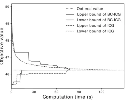
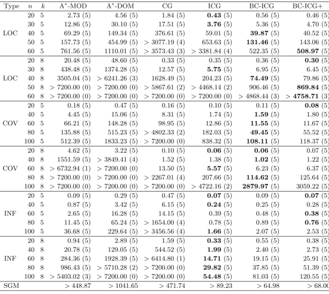
We first observed that ICG attained better results than CG for almost all classes. Fig-ure 1 represents trends of the upper and lower bounds obtained by CG and ICG with respect to the elapsed computation time for an LOC instance with n = 40, k = 8 (we used an in-stance named L.40.8.3). From Figure 1, we observed that ICG improves the lower bound as well as the upper bound. Although we have originally proposed ICG to improve the upper bounds, it also improves the lower bounds with a number of better feasible solutions than those obtained by CG. Next, Figure 2 represents trends of the upper and lower bounds obtained by ICG and BC-ICG with respect to the elapsed computation time for an LOC instance with n = 50, k = 5 (we used an instance named L.50.5.1). From Figure 2, we
Figure 2: Trends of the upper and lower bounds obtained by ICG and BC-ICG with respect to the elapsed computation time
observe that BC-ICG could obtain good lower bounds at an early stage, and also it has the strength to improve the upper bound close to the optimal value.
We observe that ICG, BC-ICG and BC-ICG+ solved optimally 138, 148 and 148 out of all 150 instances, respectively. On the other hand, A∗-MOD, A∗-DOM and CG solved optimally 124, 114 and 108 instances, respectively. Figure 3 shows performance profiles [4] of the algorithms for a parameter 1≤ γ ≤ 10. For a given set of algorithms A and instances I, the performance profile is defined in terms of computation time T (A, I) of an algorithm A ∈ A to solve an instance I ∈ I optimally. For a pair of algorithm A ∈ A and instance I ∈ I, the performance ratio R(A, I) (i.e., the ratio of computation time over the best) is defined as
R(A, I) = T (A, I) min A′∈AT (A
′, I), (4.4)
where we set R(A, I) = ∞ if none of the algorithms solved the instance I optimally. We note that R(A, I)≥ 1 holds by definition. The performance profile of an algorithm A ∈ A illustrates the function ρA(γ) that represents the number of instances I ∈ I satisfying
R(A, I) ≤ γ. From Figure 3, we observed that BC-ICG and BC-ICG+ solve almost all instances with γ = 3. We also observed that ICG solve about 120 instances optimally out of all 150 instances with γ = 3 while the conventional constraint generation (CG) solved less than 40 instances.
Table 1 also shows the shifted geometric mean [19] of the computation time of the algo-rithms in the bottom line. For an algorithm A ∈ A, the shifted geometric mean SGM(A) is defined as follows:
SGM (A) = exp (
∑ I∈I
ln (max{1, T (A, I) + shift}) |I|
)
− shift, (4.5)
where we set shift = 10 according to [19]. If an algorithm could not solve an instance opti-mally within the time limit, then we set the computation time to 7200 seconds. According to
Figure 3: Performance profiles for the algorithms
comparison of the algorithms through the shifted geometric mean of their computation time, we observed that our BC-ICG and BC-ICG+ performed better than existing algorithms.
Tables 1 and 3 show that BC-ICG and BC-ICG+ performed better than the existing algorithms, CG, A∗-MOD and A∗-DOM especially for the instances with k = 8. We observe that the A∗ search algorithms obtain upper bounds by repeatedly adding an increment fS({i}) of an element i /∈ S from the current node S until |S| = k holds. The A∗ search algorithms accordingly obtain much worse upper bounds when the size k of the cardinality constraint grows. On the other hand, our algorithms obtain upper bounds by solving reduced BIP problems with the original cardinality constraint |S| = k. Our algorithms accordingly obtain good upper bounds regardless of the size k of the cardinality constraint.
In Table 1, neither A∗-MOD, A∗-DOM, CG nor ICG could solve any of LOC instances with n = 60, k = 8. However, in Table 3, the average relative gap of ICG is much smaller than those of the others. Similarly, BC-ICG and BB-ICG+ attain good feasible solutions very close to optimal ones for a few remaining instances not optimally solved.
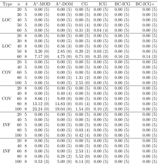
From Table 2, we observed that BC-ICG and BC-ICG+ attained optimal solutions while processing much smaller numbers of nodes than A∗-MOD and A∗-DOM. These results show that ICG attained much better upper bounds than the heuristic functions hmod and hdom for most instances and then the proposed algorithms succeeded in drastically reducing the computation time.
5. Conclusion
In this paper, we present an efficient branch-and-cut algorithm for the non-decreasing sub-modular function maximization problem based on a BIP formulation with a huge number of constraints. We propose an improved constraint generation algorithm that starts from a small subset of constraints taken from the constraints and repeats solving a reduced BIP problem while adding a promising set of constraints at each iteration. We incorporate it into a branch-and-cut algorithm to attain good upper bounds with much less computational ef-fort. According to computational results for well-known benchmark instances, our algorithm achieved better performance than the existing A∗ search algorithms and the conventional constraint generation algorithm.
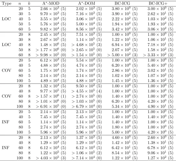
Table 1: Computation time (in seconds) of the algorithms
Type n k A∗-MOD A∗-DOM CG ICG BC-ICG BC-ICG+
20 5 2.73 (5) 4.56 (5) 1.84 (5) 0.43 (5) 0.56 (5) 0.46 (5) 30 5 12.86 (5) 30.10 (5) 17.51 (5) 3.76 (5) 5.36 (5) 4.70 (5) LOC 40 5 69.29 (5) 149.34 (5) 376.61 (5) 59.01 (5) 39.87 (5) 40.52 (5) 50 5 157.73 (5) 454.99 (5) > 3077.19 (4) 653.63 (5) 131.46 (5) 143.06 (5) 60 5 761.56 (5) 1110.01 (5) > 3573.43 (3) > 3381.84 (4) 522.35 (5) 508.97 (5) 20 8 20.48 (5) 48.60 (5) 0.33 (5) 0.35 (5) 0.36 (5) 0.30 (5) 30 8 438.48 (5) 1374.28 (5) 12.57 (5) 5.75 (5) 6.95 (5) 6.45 (5) LOC 40 8 3505.04 (5) > 6241.26 (3) 1628.49 (5) 204.23 (5) 74.49 (5) 79.86 (5) 50 8 > 7200.00 (0) > 7200.00 (0) > 5867.61 (2) > 4468.14 (2) 906.46 (5) 869.84 (5) 60 8 > 7200.00 (0) > 7200.00 (0) > 7200.00 (0) > 7200.00 (0) > 4868.44 (3) > 4758.71 (3) 20 5 0.18 (5) 0.47 (5) 0.16 (5) 0.10 (5) 0.11 (5) 0.08 (5) 40 5 4.45 (5) 15.06 (5) 8.31 (5) 1.74 (5) 1.59 (5) 1.80 (5) COV 60 5 66.21 (5) 148.28 (5) 98.95 (5) 12.86 (5) 11.55 (5) 11.67 (5) 80 5 135.88 (5) 515.23 (5) > 4802.33 (2) 182.03 (5) 49.45 (5) 55.52 (5) 100 5 512.39 (5) 1833.23 (5) > 7200.00 (0) 838.32 (5) 108.11 (5) 118.37 (5) 20 8 4.62 (5) 3.22 (5) 0.10 (5) 0.06 (5) 0.06 (5) 0.07 (5) 40 8 1551.59 (5) > 3849.41 (4) 1.52 (5) 1.38 (5) 1.02 (5) 1.22 (5) COV 60 8 > 6732.94 (1) > 7200.00 (0) 13.50 (5) 5.57 (5) 6.23 (5) 6.37 (5) 80 8 > 7200.00 (0) > 7200.00 (0) > 2267.01 (4) 207.66 (5) 114.62 (5) 125.64 (5) 100 8 > 7200.00 (0) > 7200.00 (0) > 7200.00 (0) > 4722.16 (2) 2879.97 (5) 3059.22 (5) 20 5 0.09 (5) 0.29 (5) 0.47 (5) 0.07 (5) 0.09 (5) 0.07 (5) 40 5 0.87 (5) 3.42 (5) 6.15 (5) 0.24 (5) 0.25 (5) 0.28 (5) INF 60 5 2.65 (5) 16.28 (5) 14.15 (5) 0.39 (5) 0.48 (5) 0.38 (5) 80 5 11.45 (5) 65.24 (5) > 1654.00 (4) 0.78 (5) 0.89 (5) 0.76 (5) 100 5 36.68 (5) 229.64 (5) > 3456.56 (4) 1.66 (5) 2.07 (5) 2.53 (5) 20 8 0.94 (5) 2.89 (5) 1.59 (5) 0.33 (5) 0.55 (5) 0.38 (5) 40 8 20.78 (5) 129.05 (5) 544.52 (5) 1.99 (5) 2.40 (5) 2.73 (5) INF 60 8 284.36 (5) 1928.39 (5) > 6414.80 (1) 14.71 (5) 19.15 (5) 25.91 (5) 80 8 986.43 (5) > 5710.28 (2) > 7200.00 (0) 29.82 (5) 37.85 (5) 51.39 (5) 100 8 > 5403.02 (3) > 7200.00 (0) > 7200.00 (0) 54.48 (5) 81.03 (5) 120.55 (5) SGM > 448.87 > 1041.65 > 471.74 > 89.23 > 64.98 > 68.00 References
[1] W. Chen, Y. Chen and K. Weinberger: Filtered search for submodular maximization with controllable approximation bounds. In Proceedings of the 18th International Con-ference on Artificial Intelligence and Statistics (AISTATS’15), 156–164.
[2] H. Crowder and M.W. Padberg: Solving large-scale symmetric travelling salesman problems to optimality. Management Science, 26 (1980), 495–509.
[3] A. Das and D. Kempe: Submodular meets spectral: Greedy algorithms for subset selection, sparse approximation and dictionary selection. In Proceedings of the 28th International Conference on Machine Learning (ICML’11), 1057–1064.
[4] D.E. Dolan and J.J. More: Benchmarking optimization software with performance profiles. Mathematical Programming, 91 (2002), 201–213.
[5] D. Golovin and A. Krause: Adaptive submodularity: Theory and applications in active learning and stochastic optimization. Journal of Artificial Intelligence Research, 42 (2011), 427–486.
[6] M. Gr¨otschel and O. Holland: Solution of large-scale symmetric travelling salesman problems. Mathematical Programming, 51 (1991), 141–202.
Table 2: Number of processed nodes by the algorithms
Type n k A∗-MOD A∗-DOM BC-ICG BC-ICG+
20 5 2.66× 10³ (5) 2.02× 10³(5) 3.80× 100(5) 3.00× 100(5) 30 5 9.70× 10³ (5) 7.16× 10³(5) 3.90× 101(5) 2.62× 101(5) LOC 40 5 3.55× 10⁴ (5) 3.06× 10⁴(5) 2.22× 10²(5) 1.03× 10²(5) 50 5 5.76× 10⁴ (5) 5.00× 10⁴(5) 1.94× 10²(5) 1.93× 10²(5) 60 5 9.82× 10⁴ (5) 8.56× 10⁴(5) 3.42× 10²(5) 3.06× 10²(5) 20 8 2.45× 10⁴ (5) 7.51× 10³(5) 1.00× 100(5) 1.00× 100(5) 30 8 2.67× 10⁵ (5) 1.14× 10⁵(5) 1.22× 101(5) 1.06× 101(5) LOC 40 8 1.48× 10⁶ (5) > 4.68× 10⁵(3) 6.94× 101(5) 7.18× 101(5) 50 8 > 1.77× 10⁶ (0) > 2.65× 10⁵(0) 2.07× 10²(5) 1.58× 10²(5) 60 8 > 9.98× 10⁵ (0) > 1.54× 10⁵(0) > 5.00× 10²(3) > 3.33× 10²(3) 20 5 6.12× 10² (5) 5.54× 10²(5) 1.00× 100(5) 1.00× 100(5) 40 5 4.88× 10³ (5) 4.74× 10³(5) 6.20× 100(5) 5.40× 100(5) COV 60 5 1.75× 10⁴ (5) 1.74× 10⁴(5) 2.86× 101(5) 3.02× 101(5) 80 5 2.14× 10⁴ (5) 2.14× 10⁴(5) 1.02× 10²(5) 1.07× 10²(5) 100 5 4.89× 10⁴ (5) 4.88× 10⁴(5) 1.45× 10²(5) 1.36× 10²(5) 20 8 1.32× 10⁴ (5) 9.50× 10²(5) 1.00× 100(5) 1.00× 100(5) 40 8 9.77× 10⁵ (5) > 4.55× 10⁵(4) 1.00× 100(5) 1.00× 100(5) COV 60 8 > 1.57× 10⁶ (1) > 2.74× 10⁵(0) 1.40× 100(5) 1.00× 100(5) 80 8 > 1.01× 10⁶ (0) > 1.03× 10⁵(0) 6.20× 100(5) 4.20× 100(5) 100 8 > 6.91× 10⁵ (0) > 6.79× 10⁴(0) 5.34× 101(5) 4.90× 101(5) 20 5 2.14× 10² (5) 2.13× 10²(5) 1.00× 100(5) 1.00× 100(5) 40 5 7.45× 10² (5) 7.45× 10²(5) 1.40× 100(5) 1.40× 100(5) INF 60 5 1.14× 10³ (5) 1.14× 10³(5) 1.40× 100(5) 1.00× 100(5) 80 5 2.74× 10³ (5) 2.74× 10³(5) 1.80× 100(5) 1.00× 100(5) 100 5 5.96× 10³ (5) 5.96× 10³(5) 5.00× 100(5) 4.20× 100(5) 20 8 2.13× 10³ (5) 1.37× 10³(5) 4.60× 100(5) 2.60× 100(5) 40 8 1.29× 10⁴ (5) 1.29× 10⁴(5) 1.42× 101(5) 1.38× 101(5) INF 60 8 6.12× 10⁴ (5) 6.12× 10⁴(5) 6.42× 101(5) 6.78× 101(5) 80 8 1.22× 10⁵ (5) > 1.06× 10⁵(2) 8.54× 101(5) 9.06× 101(5) 100 8 > 4.03× 10⁵ (3) > 7.14× 10⁴(0) 1.22× 10²(5) 1.27× 10²(5) [7] IBM ILOG CPLEX Optimization Studio (IBM, 2019).
https://www.ibm.com/products/ilog-cplex-optimization-studio
[8] F.H. Harper and J.A. Konstan: The MovieLens datasets: History and context. ACM Transactions on Interactive Intelligent Systems, 5-4 (2015), 1–19.
[9] A. Jovic, K. Brkic and N. Bogunovic: A review of feature selection methods with ap-plications. In Proceedings of 38th International Convention on Information and Com-munication Technology, Electronics and Microelectronics (MIPRO’15), 1200–1205. [10] Y. Kawahara, K. Nagano, K. Tsuda and J.A. Bilmes: Submodularity cuts and
appli-cations. In Proceedings of the 22nd International Conference on Neural Information Processing Systems (NIPS2009), 916–924.
[11] D. Kempe, J. Kleinberg and E. Tardos: Maximizing the spread of influence through a social network. In Proceedings of the 9th ACM SIGKDD International Conference on Knowledge Discovery and Data Mining (KDD’03), 137–146.
[12] J. Kratica, D. Tosic, V. Filipovic, I. Ljubic and P. Tolla: Solving the simple plant location problem by genetic algorithm. RAIRO-Operations Research, 35-1 (2001), 127– 142.
[13] A. Krause and D. Golovin: Submodular function maximization. In L. Bordeaux, Y. Hamadi and P. Kohli (eds.), Tractability: Practical Approaches to Hard Problems
Table 3: Relative gap (zUB− zLB)/zLB× 100 (%) of the algorithms
Type n k A∗-MOD A∗-DOM CG ICG BC-ICG BC-ICG+
20 5 0.00 (5) 0.00 (5) 0.00 (5) 0.00 (5) 0.00 (5) 0.00 (5) 30 5 0.00 (5) 0.00 (5) 0.00 (5) 0.00 (5) 0.00 (5) 0.00 (5) LOC 40 5 0.00 (5) 0.00 (5) 0.00 (5) 0.00 (5) 0.00 (5) 0.00 (5) 50 5 0.00 (5) 0.00 (5) 0.01 (4) 0.00 (5) 0.00 (5) 0.00 (5) 60 5 0.00 (5) 0.00 (5) 0.31 (3) 0.04 (4) 0.00 (5) 0.00 (5) 20 8 0.00 (5) 0.00 (5) 0.00 (5) 0.00 (5) 0.00 (5) 0.00 (5) 30 8 0.00 (5) 0.00 (5) 0.00 (5) 0.00 (5) 0.00 (5) 0.00 (5) LOC 40 8 0.00 (5) 0.56 (3) 0.00 (5) 0.00 (5) 0.00 (5) 0.00 (5) 50 8 3.26 (0) 2.85 (0) 0.20 (2) 0.03 (2) 0.00 (5) 0.00 (5) 60 8 7.17 (0) 4.75 (0) 0.71 (0) 0.35 (0) 0.16 (3) 0.14 (3) 20 5 0.00 (5) 0.00 (5) 0.00 (5) 0.00 (5) 0.00 (5) 0.00 (5) 40 5 0.00 (5) 0.00 (5) 0.00 (5) 0.00 (5) 0.00 (5) 0.00 (5) COV 60 5 0.00 (5) 0.00 (5) 0.00 (5) 0.00 (5) 0.00 (5) 0.00 (5) 80 5 0.00 (5) 0.00 (5) 1.31 (2) 0.00 (5) 0.00 (5) 0.00 (5) 100 5 0.00 (5) 0.00 (5) 2.55 (0) 0.00 (5) 0.00 (5) 0.00 (5) 20 8 0.00 (5) 0.00 (5) 0.00 (5) 0.00 (5) 0.00 (5) 0.00 (5) 40 8 0.00 (5) 0.40 (4) 0.00 (5) 0.00 (5) 0.00 (5) 0.00 (5) COV 60 8 8.66 (1) 9.89 (0) 0.00 (5) 0.00 (5) 0.00 (5) 0.00 (5) 80 8 13.12 (0) 14.83 (0) 0.01 (4) 0.00 (5) 0.00 (5) 0.00 (5) 100 8 23.24 (0) 19.04 (0) 1.54 (0) 0.10 (2) 0.00 (5) 0.00 (5) 20 5 0.00 (5) 0.00 (5) 0.00 (5) 0.00 (5) 0.00 (5) 0.00 (5) 40 5 0.00 (5) 0.00 (5) 0.00 (5) 0.00 (5) 0.00 (5) 0.00 (5) INF 60 5 0.00 (5) 0.00 (5) 0.00 (5) 0.00 (5) 0.00 (5) 0.00 (5) 80 5 0.00 (5) 0.00 (5) 0.03 (4) 0.00 (5) 0.00 (5) 0.00 (5) 100 5 0.00 (5) 0.00 (5) 0.42 (4) 0.00 (5) 0.00 (5) 0.00 (5) 20 8 0.00 (5) 0.00 (5) 0.00 (5) 0.00 (5) 0.00 (5) 0.00 (5) 40 8 0.00 (5) 0.00 (5) 0.00 (5) 0.00 (5) 0.00 (5) 0.00 (5) INF 60 8 0.00 (5) 0.00 (5) 2.53 (1) 0.00 (5) 0.00 (5) 0.00 (5) 80 8 0.00 (5) 0.28 (2) 5.52 (0) 0.00 (5) 0.00 (5) 0.00 (5) 100 8 0.53 (3) 5.00 (0) 6.14 (0) 0.00 (5) 0.00 (5) 0.00 (5)
(Cambridge University Press, 2014), 71–104.
[14] J. Lee, V.S. Mirrokni, V. Nagarajan and M. Sviridenko: Non-monotone submodular Maximization under matroid and knapsack constraints. In Proceedings of the 41st An-nual ACM Symposium on Theory of Computing (STOC’09), 323–332.
[15] H. Lin and J. Bilmes: A class of submodular functions for document summarization. In Proceedings of the 49th Annual Meeting of the Association for Computational Lin-guistics (HLT’11), 510–520.
[16] L. Lov´asz: Submodular functions and convexity. In A. Bachem, M. Gr¨otschel and B. Korte (eds.), Mathematical Programming — The State of the Art (Springer, 1983), 235–257.
[17] H. Marchand, A. Martin, R. Weismantel and L. Wolsey: Cutting planes in integer and mixed integer programming. Discrete Applied Mathematics, 123 (2002), 397–446. [18] M. Minoux: Accelerated greedy algorithms for maximizing submodular set functions.
In J. Stoer (ed.), Optimization techniques, Lecture Note in Control and Information Sciences, 7 (Springer, 1978), 234–243.
[19] H. Mittelmann, Decision tree for optimization software: Benchmarks for optimization software. http://plato.asu.edu/bench.html
[20] G.L. Nemhauser, L.A. Wolsey and M.L. Fisher: An analysis of approximations for maximizing submodular set functions I. Mathematical Programming, 14-1 (1978), 265– 294.
[21] G.L. Nemhauser and L. Wolsey: Maximizing submodular set functions: Formulations and analysis of algorithms. Studies on Graphs and Discrete Programming, 11 (1981), 279–301.
[22] S. Sakaue and M. Ishihata: Accelerated best-first search with upper-bound computation for submodular function maximization. In Proceedings of the 32nd AAAI Conference on Artificial Intelligence (AAAI-18), 1413–1421.
[23] H. Tuy: Concave programming under linear constraints. Soviet Mathematics Doklady,
5 (1964), 1437–1440.
[24] N. Uematsu, S. Umetani and Y. Kawahara: An efficient branch-and-bound algorithm for submodular function maximization. (2018). https://arxiv.org/abs/1811.04177 [25] N. Uematsu, S. Umetani and Y. Kawahara: Randomly generated test instances and
detailed computational results for submodular function maximization problem. https://sites.google.com/site/shunjiumetani/benchmark
[26] N. Uematsu, S. Umetani and Y. Kawahara: An efficient branch-and-cut
algorithm for approximately submodular function maximization. (2019).
https://arxiv.org/abs/1904.12682
[27] K. Wei, R. Iyer and J. Bilmes: Submodularity in data subset selection and active learning. In Proceedings of the 32nd International Conference on Machine Learning (ICML’15), 1954–1963.
[28] L. Yu and H. Liu: Efficient feature selection via analysis of relevance and redundancy. Journal of machine learning research, 5 (2004), 1205–1224.
A. Computational Results for Simple MIP Models
Facility location (FOC) and weighted coverage (COV) problem can be formulated as simple MIP models and directly solved by MIP solvers such as CPLEX 12.8 (see Section 4).
The facility location (LOC) problem can be formulated as the following MIP model [21].
maximize ∑ i∈M ∑ j∈N gijxij subject to ∑ j∈N xij ≤ 1, i∈ M, ∑ j∈N yj ≤ k, xij ≤ yj, i∈ M, j ∈ N, yj ∈ {0, 1}, j ∈ N, xij ∈ {0, 1}, i ∈ M, j ∈ N, (A.1)
where yj = 1 means that a facility is placed at location j ∈ N, i.e., the set of locations
S ⊆ N corresponds to a vector y = (y1, . . . , yn) satisfying yj = 1 for j ∈ S. For a given vector y, an optimal vector x is given by
xij = {
1 for some j ∈ N such that gij = max
h∈S gih
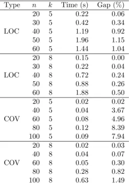
Table 4: Computation time (in seconds) and average gap (zLP− zIP)/zLP× 100 (%) of a MIP
solver (CPLEX 12.8)
Type n k Time (s) Gap (%)
20 5 0.22 0.06 30 5 0.42 0.34 LOC 40 5 1.19 0.92 50 5 1.96 1.15 60 5 1.44 1.04 20 8 0.15 0.00 30 8 0.22 0.04 LOC 40 8 0.72 0.24 50 8 0.88 0.26 60 8 1.88 0.50 20 5 0.02 0.02 40 5 0.04 3.67 COV 60 5 0.08 4.96 80 5 0.12 8.39 100 5 0.09 7.94 20 8 0.02 0.03 40 8 0.04 0.07 COV 60 8 0.05 0.30 80 8 0.28 0.82 100 8 0.63 1.49
The weighted coverage (COV) problem can be formulated as the following MIP model.
maximize ∑ i∈M wiyi subject to ∑ j∈N aijxj ≥ yi i∈ M, ∑ j∈N xj ≤ k, xj ∈ {0, 1}, j ∈ N, yi ∈ {0, 1}, i∈ M, (A.3)
where xj = 1 means that a sensor j ∈ N is selected to cover items, i.e., the set of sensors
S ⊆ N corresponds to a vector x = (x1, . . . , xn) satisfying xj = 1 for j ∈ S. For a given vecor x, an optimal vector y is given by
yi = 1 ∑ j∈N aijxj ≥ 1 0 otherwise. (A.4)
We have solved all LOC and COV instances of the above MIP models by a MIP solver (CPLEX 12.8). Table 4 shows the average computation time (in seconds) and the average gap between the optimal values of MIP and its LP relaxation (zLP−zIP)/zLP×100 (%) for each
class of instances. According to the Gap in Table 4, we can see that the MIP solver attains a good upper bound by only solving an LP relaxation of the simple MIP formulations, while the constraint generation (CG) algorithm solves many reduced BIP problems to attain the comparable upper bounds. Therefore, the simple MIP formulation is very efficient for the LOC and COV problems. However, our algorithms can solve wider class of problems, not only problems which can be formulated as simple MIP formulations.
B. Parameters for Generating Instances
We set a few parameters to generate benchmark instances differently from those of Sakaue and Ishihata [22] due to the difference between the cardinality constraint and the knapsack constraint (see Section 4).
We set a parameter p for weighted coverage (COV) instances so that a sensor j ∈ N randomly covers an item i ∈ M with probability p = 0.15, while Sakaue and Ishihata [22] originally set the parameter p = 0.3. If k× p ≥ 1 holds, then it is possible to cover all items by k sensors with high probability, and the optimal value takes trivial∑j∈Nwj for the case. We note that COV instances become rather easy for the case because the greedy algorithm often attains the optimal solutions. To make a variety of hardness for COV instances, we set the parameter p = 0.15 for satisfying k × p < 1 for COV instances with k = 5 and k× p > 1 for those with k = 8.
We set a parameter p for bipartite influence (INF) instances so that an edge (i, j)∈ A is randomly generated with probability p = 0.1, while Sakaue and Ishihata [22] originally set the parameter p = 0.3. Based on our preliminary computational experiments, INF instances become rather hard for the case with p = 0.3 under the cardinality constraint so that none of the algorithms attain an optimal solution within the time limit for those n > 50. We note that the submodular function maximization problem with the cardinality constraint tends to be harder than that with the knapsack constraint. We accordingly set the parameter p = 0.1 for INF instances.
Naoya Uematsu
RIKEN Center for Advanced Intelligence Project 6-2-3 Furuedai, Suita-shi,
Osaka 565-0874 Japan