ESRI Research Note No.34
Quality and Cost of Health Care in Japan
- Quality-Cost Trade-off and Cost-Benefit Analysis -
Shigeru Sugihara, Koichi Kawabuchi,
Yasuko Ikemoto, and Ikumi Imamura
July 2017
Economic and Social Research Institute Cabinet Office
Tokyo, Japan
The views expressed in “ESRI Research Note” are those of the authors and not those of the Economic and Social Research Institute, the Cabinet Office, or the Government of Japan. (Contact us: https://form.cao.go.jp/esri/en_opinion-0002.html)
Quality and Cost of Health Care in Japan
- Quality-Cost Trade-off and Cost-Benefit Analysis
†-
Shigeru Sugihara
‡Koichi Kawabuchi
§Yasuko Ikemoto
**Ikumi Imamura
††July 2017
† This paper was originally presented at the ESRI seminor held on 30 March, 2011. A
change of positions for one of the authors just after the meeting resulted in the delay in its revision.
‡ Social and Economic Research Institute, Cabinet Office. § Tokyo Medical and Dental University.
** Social and Economic Research Institute, Cabinet Office. †† Northern Territories Affairs Administration, Cabinet Office.
Abstract
Quality relative to cost is important in any field of economics. Health care is not an exception. If quality is superb relative to cost, it is worth incurring the cost. If quality is poor, cheap care is of little use. Cost-benefit analysis has been performed on a lot of individual treatments. It is unclear, however, whether health care expenditures of a country as a whole is worth spending specifically in Japan. Virtually no attempts are made to measure the benefits of health care for the country. We quantify the trade-off between quality and cost of health care in Japan and perform cost-benefit analysis for the country as a whole. Due to data availability, our analysis is restricted to AMI patients in a small number of hospitals. The results are suggestive, however. We find strong evidence that there is a positive trade-off: higher quality requires a higher cost, or, a lower cost induces lower quality. Whether the cost is worth it depends the value of life, of course. With the value of life of reasonable range, lower mortality more than compensates higher costs.
1. Introduction
Quality relative to cost is important in any field of economics. Health care is not an exception. If quality is superb relative to cost, it is worth incurring the cost. If quality is poor, cheap care is of little use.
Cost-benefit analysis has been performed with respect to a lot of individual treatments. It is unclear, however, whether health care expenditures of a country as a whole is worth spending specifically in Japan. Virtually no attempts are made to measure the benefits of health care for the total health system.
We quantify the trade-off between quality and cost of health care in Japan and perform a cost-benefit analysis for the care of AMI patients. Although the methods are applicable to the health care system as a whole, due to data limitation, we restrict our analysis to a small sample of Japanese hospitals.
In examining the quality-cost trade-off, it is important to recognize the endogeneity or simultaneous determination of quality and cost. A simple regression of quality on cost will generate a biased estimate of the effect of cost on quality. Basically following Timbie and Normand (2008), we will examine three models to accommodate the endogeneity: the cost-in-regression model with instrumental variables, the simultaneous equations model and the two-part model.
The structure of the paper is as follows. Section 2 gives an overview of the method and presents three types of models incorporating the endogeneity of quality and cost. Section 3 describes the data used and descriptive statistics. Sections 4, 5 and 6 estimate the cost-in-regression model, the hierarchical model and the two-part model, respectively. Section 7 concludes.
2. Methods
In examining the relationship between quality and cost, simple comparison of outcome and cost is not appropriate. Quality and cost are endogenous variables so that we should control for the endogeneity.
For example, low quality of care may manifest itself in increased complications which result in higher costs. Alternatively, low quality of care may induce early death thereby shorten length of stay which implies lower costs.
We examine three ways to model the relationship between quality and cost: cost-in-regression model with instrumental variables, the simultaneous equations model and the two-part model.
Timbie and Normand (2008) proposed three methods for combining quality and efficiency measures including univariate models, regression and cost-effectiveness analysis which uses two-part model. Our analysis follow their approach with a slight modification that we replace their univariate models with simultaneous equations model by allowing random errors of mortality and cost equations to be correlated.
Cost-effectiveness analysis:
We perform standard cost-effectiveness analysis just as Timbie and Normand (2008). Incremental net benefit is defined as change in benefits multiplied by the value of unit benefit minus change in cost.
Incremental Net Benefit = λ⋅∆E−∆C,
where λ is the value of life (quality of life), ∆E is the change in benefits and ∆C
is the change in costs. Since how much life is worth is controversial, we calculate various levels of incremental net benefits by changing the value of life.
The remainder of this section will outline the three approaches to modeling joint determination of quality and cost.
(a) Regression of quality on cost
A simple way to examine the relationship between quality and cost is to regress quality on cost. We try simultaneous estimation of mortality and cost equations instead of single mortality equation with cost as an explanatory variable. In other words, we explicitly model determination of cost in conjunction with determination of mortality. We allow correlation between error terms in mortality and cost equations.
To identify the effect of cost on mortality, we need an exogenous variable which is included in the cost equation but excluded from the mortality equation. As instrumental variables we use variables which indicate whether a hospital is participating in the DPC arrangement. As is explained below, the DPC system is analogous to the DRG system and provides a strong incentive to reduce costs.
(b) Simultaneous equations: Correlation between random effects
In this approach, we directly model joint determination of quality and cost. Cost is excluded from the mortality equation.
Figure 1 Joint Determination of Quality and Cost Correlation
There are two hospital-specific random effects, one which adversely affects outcomes and the other which increases costs. If higher costs reduce mortality, these random effects will be negatively correlated. Hence, by examining the correlation between two random effects, we can infer the quality-cost trade-off.
Simultaneous estimation of mortality and cost equations require instrumental variables to distinguish two equations. Here, again, we use variables which represent DPC statuses as instruments.
(c) Two-part model
The third way to model correlation between mortality and cost is the two-part model. The two-part model decomposes the joint distribution of mortality and cost into two parts. One is the distribution of mortality and the other the distribution of cost conditional on mortality. ) | cos ( ) ( ) cos , (yit l tit p yit p l tit yit p = ⋅
We first estimate the mortality equation and second estimate cost equation according as the patient dies or not. For each part, we estimate excess mortality and excess costs.
Since risk factors change from year to year, proper risk adjustment is needed. Risk adjustment is done by estimating a logistic regression model to measure the influence of
Choice of Treatment Quality Costs State of patient ( Risk factors )
risk factors on mortality. We re-transform the linear predictor in the logistic regression back to the probability scale for individuals. Then, we average across all patients within each year to obtain the predicted outcome.
To adjust for case mix differences across years, we follow Timbie, et al. (2009:Cost-Effectiveness paper) who adopted indirect standardization. We estimate counterfactual outcomes for each year assuming underlying quality levels of the entire population while conditioning on each year’s case mix. We take the difference between this expected outcome and the predicted outcome to yield an excess mortality for each year.
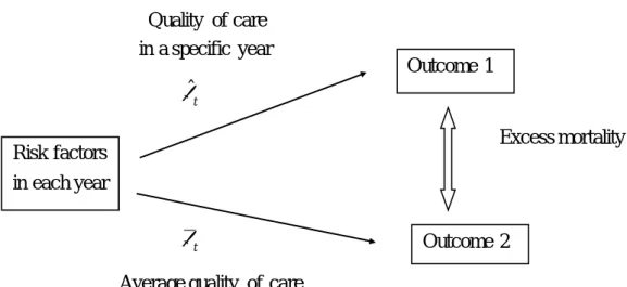
More concretely, in the indirect standardization, patient mix (distribution of risk factors) is fixed at actual mix in each year for both predicted and expected outcomes. We compare mortality rates of the following two cases for each year. Outcome 1 uses realized quality of care with the relationship between risk factors and outcome being actual one for each year. Outcome 2 uses average quality of care with the hypothetical relationship between risk factors and outcome being estimated by supposing that each year’s quality of care is the same as the total year. Then, excess mortality is calculated as the difference between two outcomes.
Figure 2 Indirect Standardization
Quality of care in a specific year βˆ t Excess mortality βt
Average quality of care Risk factors
in each year
Outcome 1
3. Data and basic statistics
Data were collected on AMI patients in 9 hospitals with a record of hospitalization at some period of time from 2004.4.1 to 2007.3.31. These hospitals had agreed to cooperate in the research for the consecutive years upon approval of in-hospital ethical committee.
We created structured questionnaires for data collection. Questionnaire I asked for detailed clinical information on the patient as well as information on the treatment the patient received. Claim data and physicians profile were collected by Questionnaire II. Questionnaire III collected overall information on AMI treatment at the hospital, such as the annual total number of CABG conducted. A part-time lecturer with physician’s license in Thoracic-Cardiovascular Surgery Section of Tokyo Medical and Dental University stayed throughout the research to fill Questionnaire I from patient medical records including nursing records and discharge summary at each hospital. Questionnaire II and III were filled by hospital staffs who were approved of the access to claim data at each hospital.
Sample is restricted to ST-Elevation AMI in the following analyses. This choice is intended to secure homogeneity in the sample as is epitomized by the separate compilation of ACC/AHA guidelines for the management of patients with ST-Elevation myocardial infarction from those for the management of patients with Non-ST-Elevation myocardial infarction.
Nine hospitals were included in the data set. Only the hospitals with more than ten STEMI patients in every year are retained in the analysis. Observations are 2631 in total, of which 598 are in 2004, 612 in 2005, 672 in 2006 and 749 in 2007.
Table 1 shows basic statistics of patients for all hospitals. The Average age is 68.9 years old and a little less than a third patients is female. About a half of patients are in the Killip class 1, a quarter in the class 2 and a little less than 15% in classes 3 and further 14% in the class 4. Occlusion of the left main trunk, left bundle branch block and ventricular fibrillation account for around 4 to 6% of patients, respectively. More than a half of patients are with hypertension and a little less than 40% and a little more than a third are with hyperlipidemia and diabetes mellitus. 8% of patients suffer from heart failure and 10% from renal failure. The share of patients with cancer is 8%. Table 2 exhibits characteristics of sample hospitals. Three out of nine hospitals are designated as tertiary critical care hospitals and all except one hospitals are designated as teaching hospitals. The average number of beds is 434. Hospitals in the sample are large in general, but the size varies. One hospital holds nearly 1000 beds while two
hospitals have less than 200 beds. The average number of AMI patients is 86, but the variation is large. Two hospitals admitted more than 150 AMI patients while two hospitals admitted only around 20. The average number of PCI performed is 297, which is a large number in the Japanese standard. Again, there is a great variation among hospitals. A hospital performed more than 700 PCI while two hospitals performed only a little more than 100 PCI.
Cost is charge billed either to the Social Insurance Funds if the medical activity is covered by the social insurance or to individuals if not. Of course, this is not a true cost, but a cost to the patients or taxpayers. The use of this concept of cost could be justified because this is the cost the society has to pay in order to obtain better quality of health care.
Figure 3 depicts crude mortality and cost over time. In 2004, crude mortality rate is a little above 9 % while mean cost is a little less than 2.6 million yen. In 2005, mean cost declined by around 0.1 million yen with a rise in mortality rate. The year 2006 saw a dramatic fall of cost to nearly 2.1 million yen together with a commensurate rise in mortality rate to more than 12 %. Then, in 2007, mortality rate declined with virtually no change in cost.
The decline in cost parallels with a decline in average length of stay (Figure 4). During this period, heavy pressures to reduce medical expenditures are felt by hospitals. The introduction of the DPC system may have been especially powerful to induce hospitals to reduce length of stay.
The Diagnosis Procedure Combination (DPC) system was introduced in 2003 as a prospective payment system for acute care of patients treated by the Specific Function Hospitals. Thereafter, the DPC system has been expanded to include other eligible hospitals. As of July 2010, the DPC system covers 1,391 hospitals and around 460,000 beds, which account for 50.4% of total beds.
The classification of patients starts with the diagnosis which absorbed resources the most among their diagnoses. Patients are further classified by whether specified operations are performed or not. Then, the final classification is reached according as whether the patient has comorbidities or not.
The DPC system is intended for use in a Prospective Payment System. But it retains characteristics of fee-for-service. For example, payments are per diem, not for
the whole hospitalization episode, and the system does not apply to operations and some other costly procedures. Therefore, it provides incentives to reduce LOS as well as incentives to increase operations. Overall, the former effect is larger than the latter effect as is verified in the estimation result of, for example, the cost-in-regression model shown in Appendix Table A1.
In 2004, of nine hospitals in the sample, one was applied the DPC system, six were in preparation for it and two were neither applied nor in preparation. In 2006, seven were applied, one was in preparation and one was neither applied nor in preparation.
Figure 5 shows crude mortality and cost by hospital. Mortality represented by bar chart differs substantially among hospitals. Hospital 3 has the highest mortality rate of more than 18 % while hospital 5 has the lowest mortality rate of only a little more than 6 %. Average cost represented by line graph also varies substantially. Hospital 9 has the highest cost of nearly 300 million yen while hospital 3 has the lowest cost of much less than 200 million yen. Overall, it seems that hospitals with higher mortality tend to have lower costs. The relationship between mortality and cost will be examined in detail below.
Risk factors used in the regressions are shown in Table 1. Risk factors include age, female, Killip classes 2, 3 and 4, occlusion of the left main trunk, Left Bundle Branch Block, ventricular fibrillation(VF), history of myocardial infarction, history of PCI, history of CABG, hypertension, diabetes mellitus, hyperlipidemia, chronic obstructive pulmonary disease (COPD), bleeding tendencies, renal failure, cerebrovascular diseases and cancer.
4. Cost-in-regression model
We start with the estimation of cost-in-regression model. Since cost is endogenous variable, we explicitly model the determination of cost and to better identify the effect of cost on mortality, we include instrumental variables in the cost equation as is explained below.
We estimate simultaneous equations for the sample of all years assuming that the impact, γ , of cost on mortality is the same for all years. Since costs are very much skewed, we take log-transformation to make them more “normal”.
1[ cos 0] 1 > + + ⋅ + ⋅ + =
∑
= ij y i ij ij k K k ij x l t c u y α β γ ij lc i ij ij k K k ij x z c v t l = +∑
⋅ + ⋅ + + = δ ϕ κ 1 cos ,where y denotes the outcome of the j-th patient in the ij i-th hospital. The outcome variable, y takes the value 1 if a patient dies during the hospitalization and 0 if she ij
survives. 1[.] represents an indicator function which takes the value 1 if the condition within the square bracket is true and 0 otherwise.
l cos denotes logarithms of costs of the j-th patient in the i-th hospital. tij
x ’s are risk factors of a patient listed above. ij
z denotes instrumental variables which sill be detailed below. ij
y i
c is an unobserved random effect specific to i-th hospital which affects y . ij
lc i
c is an analogous random effect which affects l cos tij
As was pointed out above, cost is an endogenous variable so that in the mortality
equation l cos is correlated with the error term tij u . ij
We chose to model the simultaneous determination of mortality and cost. We estimate the mortality equation and cost equation simultaneously allowing error terms
ij
u and v to be correlated. ij
To identify the impact of cost on mortality, we searched for instrumental variables
which are correlated with cost but uncorrelated with the error term, u . Variables which ij
indicate whether a hospital is participating in the DPC program should be good candidates for IVs because it can be assumed that DPC participants have strong incentives to reduce costs by way of reducing the length of stay while affecting mortality only through cost. In reality, the DPC system may induce hospitals to perform
operations more aggressively. However, the net effects can be assumed to be reduced medical expenditures. This assumption is validated by the estimation results shown below.
We have two variables which show participation in the DPC program according to differing status. “DPC preparation” indicates that the hospital is in preparation of participating in the DPC program. “DPC participation” indicates that the hospital is reimbursed by the DPC program.
Prior specifications are as follows. Correlated random intercepts are assumed to be
bivariate normal with mean zero and precision matrix Σ : −1 c ~N(0,Σ−1)
i with ≡ lc i y i i c c
c . The random effect, c , for each hospital comes from the same normal i
distribution so that shrinkage toward the overall mean is expected.
The precision matrix is assumed to follow Wishart distribution with scale matrix
Ω and 2 degrees of freedom: Σ−1 ~Wishart(Ω,2). The choice of the 2 degrees of freedom is intended to represent vague prior. Ωis, in turn, specified as I2.
The coefficient, γ, on lcost is assumed to follow a normal distribution with mean zero and variance σ : 2
) , 0 ( ~ σ2
γ N . A uniform prior on the standard deviation, σ, is adopted: σ ~ Uniform(0,100). The choice of the variance of 100 is intended to represent a diffuse prior. Gelman and Hill (2007) give a thoughtful discussion on the appropriateness of this value in the context of the logistic models or log-transformed regressors. They argue that in logistic and logarithmic regressions, typical changes in outcomes are on the scale of 0.1 or 1, but not 10 or 100, so that one would not expect to see coefficients much higher than 10 in absolute values as long as the regressors are also on a reasonable scale. Although their choice of the value of variance is 2
100 , we believe that their argument applies to our choice, 100. In fact, mean estimates of γ obtained below is -0.82.
The model was estimated with Markov chain Monte Carlo methods using WinBUGS software. To check the convergence, three parallel chains were run to calculate the Gelman-Rubin statistic. A burn-in of 10,000 iterations for each chain was allowed for the model to converge. Additional 20,000 samples for each chain were drawn from the joint posterior distribution for the estimation of all model parameters.
Table 2 shows estimate of the coefficient on cost. Full results are in Appendix Table A1. The mean is -0.820 and the standard error is 0.092. The 95 % credible interval
is from -1.006 to -0.643. The probability of the coefficient being positive is zero. Hence, it is very likely that higher cost reduces mortality.
From 2004 to 2007, the average cost decreased by 16.9 % which corresponds to a decline of around 432 thousand yen. Plugging this change into the mortality equation reveals that this decline in costs raised mortality rate (i.e. reduced survival rate) by 0.57 % points from 9.20 % to 9.76 %. (The actual mortality rate increased to 10.8 %, which is influenced by random fluctuations and factors other than decreased costs.)
We can perform incremental cost-benefit analysis from this relationship. Recall the following formula:
Incremental Net Benefit = λ⋅∆E−∆C,
where λ is the value of life, ∆E is incremental benefit (change in survival rate) and
C
∆ is incremental cost.
First, we calculate the break-even value of life, which is the critical value of λ that equates the incremental gross benefit and incremental costs. We reversed the signs of the actual changes in survival rate and costs so that ∆E=+0.57% increase in survival rate corresponding to ∆C=432,042 yen increase in costs. INB is calculated as E C ∆ ∆ = * λ 005658 . 0 432042 = = 76,357 thousand yen.
Hence, if we value life at around 76.4 million yen, a 432 thousand-yen increase in costs is compensated by a 0.57 % increase in survival rate (decrease in mortality rate). If we value life more than 76.4 million yen, the 0.57 % increase in mortality more than compensate the 432 thousand-yen increase in costs.
Second, we estimate incremental net benefits according as the value of life changes. How much life is worth is controversial, at best. It is nearly impossible to pin down exact value of life, although Viscusi and Aldy(2007) find that half of the studies of the U.S. labor market reveal a value of a statistical life ranges from $5 million to $12 million and the median is $7 million when converted into year 2000 dollars. (In terms of yen, the range is from 550 million yen to 1 billion and 320 million yen with a median of 770 million yen at the exchange rate of 110 yen per dollar.) Therefore, it is common to
calculate incremental net benefits by changing the value of life.
We can draw a diagram which shows the incremental net benefit as a function of the value of life. Figure 6 shows this relationship between the value of life and incremental net benefit. As the value of life increases, the net benefit from an increase in costs and corresponding decrease in mortality (increase in survival rate) becomes larger.
5. Simultaneous equations model
In this approach, we directly model joint determination of quality and cost. Compared with the cost-in-regression model, cost is excluded from the mortality equation. For t-th
year, we checked correlation between y t
c and c in the mortality and cost equations. tlc
The outcome variable, yit, takes the value one if a patient i in time t dies and zero
if she is discharged alive.
] 0 [ 1 1 > + + ⋅ + =
∑
= it y t it k K k it x c u y α β it lc t it it k K k it x z c v t l = +∑
⋅ + ⋅ + + = δ ϕ κ 1 cosSince costs are very much skewed, we take log-transformation to make them more “normal”. Notations for variables are the same as the cost-in-regression model. Instrumental variables are also the same.
The model was estimated with Markov chain Monte Carlo methods using WinBUGS software. The number of chains, check of convergence, burn-in and samples for estimation are the same as the cost-in-regression model.
Prior specifications are also similar. Namely, correlated random intercepts are assumed to be bivariate normal with mean zero and precision matrix Σ : −1
) , 0 ( ~ N Σ−1 ct with ≡ lc t y t t c c
c . The random effect, c , for each year comes from the t
same normal distribution so that shrinkage toward the overall mean is expected.
The precision matrix is assumed to follow Wishart distribution with scale matrix
Results of the estimation of simultaneous equations model are shown in Appendix Table A2. The upper part of Table 3 presents overall correlation between random effects for mortality and those for cost. The estimate is almost zero. This is because correlations within each year are very low, which are shown in the lower part of the table.
Correlation among years seems to be high as is depicted in Figure 7. One can see negative relationship between mortality random effects and cost random effects. Overall picture is the similar to Figure 3 of crude mortality and cost. A remarkable difference is that mortality random effect in 2005 is lower than that in 2004. Estimates of random effects are after adjustment for risk factors.
The case of hospital random effects
As an alternative viewpoint, we checked the correlation between hospital random effects of mortality and cost for hospital. Namely, for i-th hospital and j-th patient, we
checked correlation between y i
c and lc
i
c in the mortality and cost equations.
] 0 [ 1 1 > + + ⋅ + =
∑
= ij y i ij k K k ij x c u y α β ij lc i ij ij k K k ij x z c v t l = +∑
⋅ + ⋅ + + = δ ϕ κ 1 cosWhen we replace year random effects with hospital random effects in the estimation of the simultaneous equations model, we obtain correlation between mortality and cost random effects of hospitals. Full results are shown in Appendix Table A2.
The upper part of Table 4 shows overall correlation. Again, the correlation is low and this is because of low correlation within hospital. Once again, correlation among hospitals seems to be high. A clear downward-sloping line is observable in Figure 8. This line would represent the trade-off between mortality and cost. Rather surprisingly, almost all hospitals lie on the line although hospitals 4 and 5 may have slightly better survival rate with lower costs.
How much confidence can we place on these estimates of random effects? Figure 9 shows mean level of random effects for mortality together with 95 % credible intervals. These random effects are not exponentiated. Overall, mortality random effects are significantly above or below zero. The probability that the random effect is above zero
is shown at the bottom of the figure. Except hospitals 3, 7 and 9, the probabilities are more than 0.9 or less than 0.1.
Figure 11 shows mean level of random effects for cost together with 95 % credible intervals. Cost random effects are above or below zero less significantly than mortality random effects. The probability that the random effect is above zero is again shown at the bottom of the figure. Four hospitals out of nine have probabilities more than 0.9 or less than 0.1 and the probabilities of other hospitals are not so different from these.
6. Two-part model
The two-part model decomposes the joint distribution of mortality and cost into two parts. One is the distribution of mortality and the other the distribution of cost conditional on mortality. ) | cos ( ) ( ) cos , (yit l tit p yit p l tit yit p = ⋅
The outcome variable, yit, takes the value one if a patient i in time t dies and zero if
she survives. We proceed in following steps.
First, as for the p(yit) part, we estimate the mortality equation:
logit[p(yit =1|xit)]=αt +βt⋅xit,
where xit is severity index. We follow Timbie, et al. (2008:Cost-Effectiveness paper) in creating a measure of disease severity, severity index, for each patient. A logistic regression was used to model the effect of demographic and clinical risk factors on in-hospital mortality. Risk factors are selected by checking statistical significance and signs of estimated coefficients. Risk factors are the same as those used in the cost-in-regression model or the simultaneous equations model. Estimation result is shown in Appendix Table A3. The severity index is estimated as a linear predictor using
the coefficients from the estimated logistic regression:
∑
= ⋅ = P p itp p it x severity 1 ˆ β , where itp
Then, we obtain predicted mortality. ) ( ) exp( 1 ) exp( ) | 1 ( t t it it t t it t t it it x x x x y p ≡Λ + ⋅ ⋅ + + ⋅ + = = α β β α β α ,
Second, as for the p(lcostit |yit) part, we estimate cost equations separately according as yit =1or 0.
lcostit =κ+ϕ⋅xit +δ⋅zit +vit
Since costs are very much skewed, we take log-transformation to make them more “normal”. We should be careful when retransforming log-cost into the original scale because expected log-cost is not equal to log of expected cost. We utilize smearing estimator proposed by Duan (1983) just as Timbie and Normand (2008).
The model was estimated with Markov chain Monte Carlo methods using WinBUGS software. The number of chains, check of convergence, burn-in and samples for estimation are the same as the cost-in-regression model.
Prior specifications are as follows. Two random effects are assumed to follow bivariate
normal with mean µ and precision matrix Σ : −1 c ~N(µ,Σ−1)
t with ≡ t t t c β α . The
random effect, c , for each year comes from the same normal distribution so that t
shrinkage toward the overall mean is expected.
Overall mean, µ , is assumed to follow a normal distribution with mean 0 and variance 100: µ~ N(0,100). The precision matrix is assumed to follow Wishart distribution with scale matrix Ω and 2 degrees of freedom: Σ−1 ~Wishart(Ω,2). The choice of the 2 degrees of freedom is intended to represent vague prior. Ωis, in turn, specified as I2.
Now, we give a detailed account of indirect standardization. As is explained above, we compare mortality rates of the following two cases for each year: Outcome 1 which uses realized quality of care and Outcome 2 which uses average quality of care.
(i) Estimation of the mortality equation: Indirect standardization
First, we estimate the mortality equation adjusting for risk factors by indirect standardization. To standardize case mixes, we compared two outcomes, actual and hypothetical.
Outcome 1 utilizes actual relationship between risk factors and outcome for each year so that parameters are estimated using the sample of each year separately. Parameters, αt and βt, depend on time t.
We estimate a logit regression model for each year,
logit[p(yit =1|xit)]=αt +βt⋅xit
to obtain estimates, αˆt and βˆt. We re-transform back into the original probability
scale: ( ) ) exp( 1 ) exp( ) | 1 ( t t it it t t it t t it it x x x x y p ≡Λ + ⋅ ⋅ + + ⋅ + = = α β β α β α .
Then, we average individual probabilities of death for each year: t = 2004, 2005, 2006 and 2007. ) ˆ ˆ ( 1 ˆ 1 it t t n i t t x n D t ⋅ + Λ =
∑
= β αThen survival rate is Eˆt =1−Dˆt.
Outcome 2 sets up a hypothetical relationship between risk factors and outcome for each year by supposing that each year’s quality of care is the same as the total year. Parameters are estimated using the sample from all years so that parameters, α and β,
do not depend on t: common parameters for all years. We estimate a logit regression model for all years,
logit[p(yit =1|xit)]=α+β⋅xit
to obtain estimates, α and β . We re-transform back into the original probability scale: p(yit =1|xit)=Λ(α +β ⋅xit).
Again, we average individual probabilities for each year: t = 2004, 2005, 2006 and 2007. ) ( 1 1 it n i t t x n D t ⋅ + Λ =
∑
= β αThen survival rate is Et = 1−Dt.
Excess mortality is the difference between Outcome 1 and Outcome 2, Eˆt − E . t
The first column of Table 5 shows the incremental benefit derived from the estimated excess mortality for each year and from 2004 to 2007.
Incremental benefit is a small positive in 2005, a large negative in 2006 and a moderate positive in 2007.
From 2004 to 2007, the incremental benefit is slight negative.
(ii) Estimation of cost equations separately according as yit =0 or 1.
Second, we estimate cost equations conditional on whether the patient died or not.
it it t t it x v t lcos =κ +ϕ ⋅ +
(a) Corresponding to yit =1: Expirer Case1: Use realized quality of care
Parameters, κˆ1t and ϕˆ1t, are estimated using the sample of each year separately. By re-transforming the estimated log-cost, lcost1it = ˆ1t + ˆ1t⋅x1it
∧
ϕ
κ , into the original scale and averaging, we obtain for each year, t = 2004, 2005, 2006, 2007,
) ˆ ˆ ( 1 ˆ 1 1 1 1 1 1 1 it t t n i t t x n C t ⋅ + =
∑
= ϕ κnatural scale, smearing estimator is applied to avoid biases due to non-linearity of log-transformation.
Suppose that cost is log-transformed, lcosti =log(costi), and the model is i
i
i x u
t
lcos =κ+ϕ⋅ + . The expected cost of individual 0 is, even with E(u|x)=0, E(cost0 |x0)=E[exp(κ+ϕ⋅x0+u)]≠exp(κ+ϕ⋅x0)
Smearing estimator proposed by Duan (1983) is:
(cos | ) [exp(ˆ ˆ ˆ)] 1 exp(ˆ ˆ 0 ˆ )
1 0 0 0 i n i i x u n u x E x t E = + ⋅ + =
∑
+ ⋅ + = ϕ κ ϕ κ , where uˆi ≡lcosti −(κˆ+ϕˆ⋅xi)Case2: Use average quality of care: Common parameters
Parameters are estimated using the sample of all years to obtain κ1 and ϕ1. Then, it
it x
t
lcos 1 =κ1+ϕ1⋅ 1 . We re-transform back to the original scale using smearing
estimator. Finally, we average for each year: t = 2004, 2005, 2006 and 2007.
) ( 1 1 1 1 1 1 1 1 1 t it n i t t x u n C t + ⋅ + =
∑
= ϕ κ (b) Corresponding to yit =0: Survivor Case1: Use realized quality of careParameters, κˆ0t and ϕˆ0t, are estimated using the sample of each year separately. By re-transforming the estimated log-cost, lcost0it = ˆ0t + ˆ0t⋅x0it
∧
ϕ
κ , into the original scale and averaging, we obtain for each year, t = 2004, 2005, 2006, 2007,
) ˆ ˆ ( 1 ˆ 0 0 0 1 0 0 0 it t t n i t t x n C t ⋅ + =
∑
= ϕ κCase2: Use average quality of care
Parameters are estimated using the sample of all years to obtain κ0 and ϕ0. Then, it
it x
t
estimator. Finally, we average the re-transformed costs for each year: t = 2004, 2005, 2006 and 2007. ) ( 1 0 0 0 1 0 0 0 it n i t t x n C t ⋅ + =
∑
= ϕ κExcess cost is weighted average of costs for expirers or survivors with mortality rates as weights. ) ˆ 1 ( ˆ ˆ ˆ 0 1t t t t t C E C E C = × + × − ∆ −{C1t×Et +C0t×(1−Et)}
Excess mortality and excess cost calculated from the two-part model are shown in Figure 11. Overall picture is similar to Figure 7 which shows year random effects in the simultaneous equation model with a main difference being that excess mortality in 2007 is below zero.
We can perform incremental cost-benefit analysis using estimates from this relationship. Recall that the following formula.
Incremental Net Benefit = λ⋅∆E−∆C,
where λ is the value of life, ∆E is incremental benefit (change in survival) and ∆C
is incremental cost. The excess survival rate decreased from 0.21% in 2004 to 0.05% in 2007. The excess cost decreased from 253562 yen in 2004 to -184646 yen in 2007. The change in the excess survival is 0.16 % while the change in the excess cost is 438,208 yen resulting in the break-even value of life of 2billion and 7810 million yen (27.8 million dollar).
7. Conclusion
This paper quantitatively examined the trade-off between quality and cost of health care in Japan and performed cost-benefit analysis for the country as a whole. Due to data
availability, our analysis was restricted to AMI patients in a small number of hospitals. The results are suggestive, however. We find strong evidence that there is a positive trade-off: higher quality requires a higher cost, or, a lower cost induces lower quality. Whether the cost is worth it depends the value of life, of course. With the value of life of reasonable range, lower mortality more than compensates higher costs.
In the sequel of this paper, we are planning to investigate into the determinants of quality of care. From our data, quality measures can be calculated for each hospital such as Door-to-Balloon time and drug therapies at arrival or discharge. By contrasting quality measures and quality of each hospital, we can examine the question: what determines the quality? For example, Figure 12 shows the relationship between Door-to-Balloon time and hospital-specific random effects for mortality. Whether quality measures are related to outcomes are hotly debated. A small sample of the literature includes Granger, et al. (2005), Bradley, et al. (2006) and Peterson, et al. (2006). Only after we identify the determinants of quality of care can we take steps to improve the quality of health care.
Quality-cost trade-off and cost-benefit analysis are similar but not identical to the concept of productivity. We are planning to measure productivity of health care more in line with economics tradition as proposed by Castelli, et al. (forthcoming).
References
Abraham, Katharine G., and Christopher Mackie, eds. (2005) Beyond the Mark et: Designing
Nonmark et Accounts for the United States. National Academies Panel on Conceptual, Measurement
and Other Statistical Issues in Developing Cost-of-Liv ing Indexes. Washington, DC: The National Academies Press for the National Research Council.
Aizcorbe, Ana, Bonnie Retus and Shelly Smith. (2007) Toward a Health Care Satellite Account.
Survey of Current Business, May 2007.
Atkinson, Tony (2005) Atk inson Review: Final Report. Measurement of Government Output and
Productivity for the National Accounts.
Aiguilar, Oma r, and Mike West. (1999) Analysis of Hospital Quality Monitors Using Hierarchical Time Series Models. In C. Gatsonis, et al., eds., Case Studies in Bayesian Statistics, vol.9, pp.287-302.
Berndt, Ernst R., Susan H. Busch and Richard G. Frank. (2001) Treatment Price Indexes for Acute Phase Major Depression. In David Cutler and Ernst Berndt, eds. Medical Care Output and
Productivity, University of Chicago Press, pp.463-505.
Berndt, Ernst, David Cutler, Richard Frank, Zvi Griliches, Joseph Newhouse and Jack Triplett. (2001) Price Indexes for Medical Care Goods and Service: An Overview of Measurement Issues. In David Cutler and Ernst Berndt, eds. Medical Care Output and Productivity, University of Chicago Press, pp.141-198.
Birkmeyer JD, Siewers AE, Finlayson EVA, Stukel TA, Lucas FL, Batista I, Welch HG, Wennberg DE Birkmeyer JD, Siewers AE, Finlayson EVA, Stukel TA, Lucas FL, Batista I, Welch HG, Wennberg DE. (2002) Hospital Volu me and Surgical Mortality in the United States. New England
Journal of Medicine 346:1128-1137.
Birkmeyer JD, Stukel TA, Siewe rs AE, Goodney PP, Wennberg DE, Lucas FL. (2003) Surgeon Vo lume and Operative Mortality in the United States. New England Journal of Medicine 349:2117-2127.
Spertus JA, Krumholz HM. Hospital quality for acute myocardial infarction: correlat ion among process measures and relationship with short-term mortality. Journal of the American Medical
Association 2006; 296:72–78.
Bronskill, Susan, Sharon-Lise Normand, Mary Landrum and Robert Rosenheck. (2002) Longitudinal Profiles of Health Care Providers. Statistics in Medicine 21: 1067-1088.
Burgess, James, Cindy Christiansen, Sarah Michalak and Ca rl Morris. (2003) Medical profiling: improving standards and risk adjustments using hierarchical models. Journal of Health Economics,
19(3): 291-309.
Carey, K., Burgess, J.: On measuring the hospital cost/quality trade-off. Health Economics 8, 509–520 (1999)
Castelli, Adriana, Diane Dawson, Hugh Gravelle and Andrew Street. (2007) Improving the Measurement of Health System Output Growth. Health Economics 16: 1091-1107.
Castelli, Adriana, Mauro Laudicella and Andrew Street. (2008) Measuring NHS Output Growth
CHE Research Paper 43, Centre for Health Economics, University of York.
Castelli A, Laudicella M, Street A, Ward P. Getting out what we put in: productivity of the English NHS. Health Economics, Policy and Law; Forthcoming.
Cle ment, J.P., Va ld manis, V.G., Ba zzoli, G.J., Zhao, M., Chukma itov, A.: Is more better? An analysis of hospital outcomes and efficiency with a DEA model of output congestion. Health Care
Management Science 11, 67–77 (2008)
Cutler, David and Ernst Berndt, eds. (2001) Medical Care Output and Productivity, University of Chicago Press.
Cutler, David and Mark McCle llan. (2001) Is Technological Change in Medicine Worth IT? Health
Affairs 20(5): 11-29.
Cutler, David, Mark McClellan, Joseph Newhouse and Dahlia Remler. (1998) Are Medical Prices Declin ing? Evidence from Heart Attack Treatment. Quarterly Journal of Economics 113(4): 991-1024.
Cutler, David, Mark McCle llan, and Joseph P. Newhouse. (1999) The Costs and Benefits of Intensive Treatment for Ca rdiovascular Disease. In Jack Trip lett, ed., Measuring the Prices of
Medical Treatments, Washington, D.C.: The Brookings Institution, 34-71.
Cutler, David M., and Elizabeth Richardson. (1999) Your Money and Your Life: The Value of Health and What Affects It. In Alan M. Garber ed., Frontiers in Health Policy Research, Vol. 2, Cambridge, MA: MIT Press, pp. 99-132.
Cutler, David, Allison Rosen and Sandeep Vijan. (2006) The Va lue of Medical Spending in the U.S., 1960-2000. New England Journal of Medicine 355(9): 920-927.
Daniels MJ, Gatsonis C. (1999) Hierarchica l generalized linear models in the analysis of variations in health care utilization. Journal of the American Statistical Association 94(445):29–42.
Daniels MJ, Normand SLT. (2006) Longitudinal profiling of health care units based on continuous and discrete patient outcomes. Biostatistics 7(1):1–15.
Dawson D, Gravelle H, O'Mahony M, Street A, Weale M, Castelli A, Jacobs R, Kind P, Loveridge P, Martin S, Stevens P and Stokes L. Developing new approaches to measuring NHS outputs and productivity. Centre for Health Economics, University of York; CHE Research Paper 6; 2005.
Draper, David, and Mark Gittoes. (2004) Statistical analysis of performance indicators in UK higher education. Journal of the Royal Statististical Society series A, 167, Part3, pp. 449–474.
Duan, N. (1983) Smearing estimates. Journal of the American Statistical Association 78: 605-610.
Evans, David, Ajay Tandon, Christopher Murray and Jeremy Lauer. (2000) The Comparative Efficiency of National Health Systems in Producing Health: An Analysis of 191 Countries. GPE Discussion Paper, No.29, World Health Organization.
Fisher, Elliott S., David E. Wennberg, Thérèse A. Stukel, Danie l J. Gottlieb, F. L. Lucas, and Étoile L. Pinder. (2003) The Implications of Regional Variat ions in Medicare Spending. Part 1: The Content, Quality, and Accessibility of Care. Part 1, Annals of Internal Medicine, Feb 2003; 138: 273 - 287. Part 2, Ann Intern Med, Feb 2003; 138: 288 - 298.
Ford, Earl S., Umed A. Ajani, Janet B. Croft, et al. (2007) Explaining the Decrease in U.S. Deaths from Coronary Disease, 1980–2000. New England Journal of Medicine 356: 2388-2399.
Fukui, Tadashi and Yasushi Iwamoto. (2004) Medical Spending and the Health Outcome of the Japanese Population. A paper for ESRI International Joint Research Project.
Garber, Alan, and Jonathan Skinner. (2008) Is American Health Care Uniquely Inefficient? Journal
of Economic Perspectives 22(4): 27-50.
Gelman, Andrew, and Jennifer Hill. (2007) Data Analysis Using Regression and
Multilevel/Hierarchical Models. Cambridge University Press.
Go ldstein, Harvey, and David Spiegelhalter. (1996) League Tables and Their Limitations: Statistical Issues in Co mparisons of Institutional Performance. Journal of the Royal Statistical Society Series A 159: 385-443.
Granger CB, Steg PG, Peterson E, et a l. (2005) Medication performance measures and mortality following acute coronary syndromes. American Journal of Medicine 118:858-865.
Greene, Willia m. (2005) Reconsidering Heterogeneity in Panel Data estimators of the Stochastic Frontier Model. Journal of Econometrics 126: 269-303.
Hvenegaard A, Nie lsen Arendt J, Street A, Gyrd-Hansen D. (2010) Exp loring the relationship between costs and quality: Does the joint evaluation of costs and quality alter the ranking of Danish hospital departments? European Journal of Health Economics
Hannan EL, O’Donnell JF, Kilburn H Jr, Bernard HR, Yazici A. (1989) Investigation of the relationship between volume and mortality for surgical procedures performed in New York State hospitals. Journal of the American Medical Association 262:503-510.
Halm, Ethan, Clare Lee and Mark Chassin. (2000) How Is Volume Related to Quality in Health Care? A Systematic Review of the Research Literature. In Interpreting the Volume-Outcome Relationship in the Context of Health Care Quality. Maria Hewitt for the Committee on the Quality of Health Care in America and the National Cancer Policy Board. Wachington DC: Institute of Medicine, National Academy Press.
Health Care. Health Care Management Science 6: 203–218.
Hollingsworth, B.: The measurement of efficiency and productivity of health care delivery. Health
Economics 17, 1107–1128 (2008)
Jacobs R, Smith PC, Street A. Measuring Efficiency in Health Care: Analytic Techniques and Health
Policy. Cambridge University Press, 2006.
Kawabuchi, Koichi, and Shigeru Sugihara. (2006) Vo lume -Outcome Re lationship in Japan: the Case of Percutaneous Transluminal Coronary Angioplasty (PTCA) Volu me on Mortality of Acute Myocardial Infarction (AMI) Patients. In David Wise and Naohiro Yashiro, eds., Health Care Issues
in the United States and Japan (National Bureau of Economic Research Conference Report),
University of Chicago Press, 2006, pp.113-145.
Kru mholz HM, Wang Y, Mattera JA, et al. (2006) An administrative claims model suitable for profiling hospital performance based upon 30-day mortality rates among patients with an acute myocardial infarction. Circulation 113:1683-1692.
Landrum MB, Bronskill SE, Normand S-LT. (2000) Analytic methods for constructing cross-sectional profiles of health care providers. Health Services and Outcomes Research
Methodology 1(1):23–47.
Landrum, Mary, Sharon-Lise Normand and Robert Rosenheck. (2003) Selection of Re lated Multivariate Means: Monitoring Psychiatric Care in the Department of Veterans Affairs. Journal of
the American Statistical Association 98: 7-16.
Luciano, Mariagrazia. (2006) Measurement of non-market output in education. Paper prepared for the joint OECD/ONS/Government of Norway workshop ”Measurement of non-market output in education and health” London, Brunei Gallery, October 3 – 5, 2006.
Marshall, Cla re, and David Spiegelhalter. (2001) Institutional Performance. In Alastair Leyland and Harvey Goldstein, eds., Multilevel Modelling of Health Statistics. John Wiley & Sons, pp.127-142.
Mark B. Mc Cle llan. (1997) Hospital Reimbursement Incentives: An Empirical Analysis. Journal of
McClellan, Mark, Barbara J. McNeil, and Joseph P. Newhouse. (1994) Does More Intensive Treatment of Acute Myocardial Infarction Reduce Mortality? Journal of the American Medical
Association, 272(11): 859-866.
McClellan, Mark and Douglas Staiger. (1999) The Quality of Health Care Providers. NBER Working Paper No.7327.
McClellan, Mark and Douglas Staiger. (2000) Comparing the Quality of Hea lth Care Providers.In Alan Garber (ed.) Frontiers in Health Policy Research, Volu me 3. 2000, The MIT Press, Ca mbridge MA, pp. 113-136.
McKay, N.L., De ily, M.E. (2008) Cost inefficiency and hospital health outcomes. Health Economics 17, 833–848.
Morey, R.C., Fine, D.J., Loree, S.W., Retzlaff-Roberts, D.L., Tsubakitani, S. (1992) The trade-off between hospital cost and quality of care. An exploratory empirical analysis. Medical Care 30, 677–698.
Murphy, Kevin M. and Robert H. Topel (2006) “The Value of Health and Longevity,” Journal of
Political Economy, Vol. 114, pp. 871–904.
Murray, Christophe, and David Evans, eds. (2003) Health Systems Performance Assessment: Debates, Methods and Empiricism. World Health Organization.
National Research Council. (2008) Strategies for a BEA Satellite Health Care Account. Summary of a Workshop, National Academies Press.
Nordhaus, William D. 2003. “The Health of Nations: The Contribution of Improved Health to Living Standards.” In Measuring the Gains from Medical Research: An Economic Approach, edited by Kevin M. Murphy and Robert H. Topel. Chicago: Univ. Chicago Press.
Normand SLT, Glic kman ME, Gatsonis CA. (1997) Statistical methods for profiling providers of medica l care : issues and applications. Journal of the American Statistical Association 92(439):803–814.
O’Hagan A, Stevens JW. (2001) A fra me work for cost-effectiveness analysis from c lin ical tria l data.
Health Economics 10:303–315.
Orosz, Eva. (2005) The OECD System of Health Accounts and the US National Hea lth Accounts: Improving Connections through Shared Expe riences. Paper Prepared for the conference on “Adapting National Health Expenditure Accounting to a Changing Health Care environment”. Centers for Medicare and Medicaid Services, 21-22 April 2005.
Orosz, Eva, and David Morgan. (2004) SHA-Based Bational Health Accounts in Thirteen OECD Countries: A Comparative Analysis. OECD Health Working Papers No.16.
Peterson ED, Rose MT, Mulgund J, et al. (2006) Association between hospital process performance and outcomes among patients with acute coronary syndrome. JAMA 295:1912-1920.
Rosen, Allison, and David Cutler. (2007) Measuring Medical Care Productivity: A Proposal for U.S. National Health Accounts. Survey of Current Business, June 2007.
Skinner, Jonathan, Elliott Fisher and John Wennberg. (2005) The Effic iency of Medicare. In David Wise, ed., Analyses in the Economics of Aging, pp. 129 – 160.
Skinner, Jonathan, and Douglas Staiger. (2009) Technology Diffusion and Productivity Growth in Health Care. NBER Working Paper No. 14865.
Skinner, Jonathan , Douglas Staiger and Elliott Fisher. (2006) Is Technological Change in Medicine Always Worth It? The Case of Acute Myocardial Infarction. Health Affairs, 25(2): w34-w47.
Smith, Peter, and Andrew Street. (2006) Analysis of Secondary School Efficiency: Final Report. Research Report No.788, Department of Education and Skill, UK.
Smith, Peter. (2006) Public Services: Are Composite Measures a Robust Reflection of Performance in the Public Sector, CHE Research Paper 16, Centre for Health Economics, University of York.
Spertus, John A., Martha J. Radford, Nathan R. Every, et al. (2003) Challenges and Opportunities in Quantifying the Quality of Care for Acute Myocardial Infarction. Circulation, vol.107, pp.1681-1691.
Spiegelhalter, David, Abrams, Keith R., Myles, Jonathan P. (2004) Bayesian Approaches to Clinical
Trials and Health Care. John Wiley & Sons.
Spiegelhalter DJ, Tho mas A, Best NG, Gilks WR. (1996) BUGS: Bayesian Inference Using Gibbs
Sampling.
Staiger, D. O., J. B. Dimick, O. Baser, Z. Fan, and J. D. Birkmeyer. (2009) Empirica lly derived composite measures of surgical performance. Medical Care 47(2):226-233.
Street A, Hakkinen U. Health system productivity and efficiency. In: Smith PC, Mossialos E, Leatherman S, Papanicolas IN, editors. Performance measurement for health system improvement: experiences, challenges and prospects: World Health Organization; 2009.
Street A, Scheller-Kre insen D, Geissler A, Busse R (2010): Determinants of hospital costs and performance variation: Methods, models and variables for the EuroDRG pro ject. Working Papers in Health Policy and Management Vol. 3 May 2010, Berlin: Universitätsverlag der TU Berlin.
Street A, Dawson D (2002) Costing Hospital Activity: the Experience with Healthcare Resources Groups in England. European Journal of Health Economics 3: 3-9.
Stewart, Susan, Rebecca Woodward, Allison Rosen and David Cutler. (2007) A Proposal for Monitoring Symptoms, Impairments and Health Ratings. NBER Working Paper No.11358.
Justin Timbie , Joseph Newhouse, Meredith Rosenthal, Sharon-Lise Normand. (2008) A Cost-Effectiveness Frame work for Profiling the Value of Hospital Care. Medical Decision Making 28: 419-434.
Justin W. Timbie , David M. Shahian, Joseph P. Newhouse, Meredith B. Rosenthal and Sharon-Lise T. Normand. (2009) Co mposite measures for hospital quality using quality-adjusted life years. Statistics
in Medicine 28:1238–1254
Justin W. Timb ie and Sharon-Lise T. Normand. (2008) A comparison of methods for combining quality and efficiency performance measures: Profiling the value of hospital care
Triplett, Jack. (2000) What’s Different about Health? In David Cutler and Ernst Berndt, eds. Medical
Care Output and Productivity, University of Chicago Press, pp.15-94.
UK Department of Health. (2005) Healthcare Output and Productivity: Accounting for Quality
Change.
UK Office for National Statistics. (2008) Sources and Methods for Public Service Productivity:
Health.
UK Office for National Statistics. (2008) Public Service Productivity.
Viscusi W, Aldy J. (2003) The value of a statistical life: a c ritica l review of ma rket estimates 504 throughout the world. Journal of Risk and Uncertainty, vol. 27(1), pages 5-76.
Weintraub, Willia m, Willia m Boden, Zugini Zhang, et al. (2008) Cost-Effectiveness of Percutaneous Coronary Intervention in Optimally Treated Stable Coronary Patients. Circulation Cardiovascular
Quality and Outcomes 1: 12-20.
Killip4 0.135 0.151 0.163 0.125 0.107
Left main trunk occluded 0.051 0.042 0.052 0.058 0.052
LBBB 0.067 0.057 0.072 0.061 0.075 Ventricular fibrillation 0.044 0.030 0.031 0.064 0.048 Hypertension 0.539 0.587 0.565 0.487 0.525 Hyperlipidemia 0.375 0.375 0.355 0.360 0.405 Diabetes mellitus 0.348 0.370 0.364 0.351 0.314 Heart failure 0.078 0.100 0.078 0.063 0.075
History of myocardial infarction 0.108 0.100 0.127 0.112 0.093
History of PCI 0.095 0.107 0.101 0.095 0.081 History of CABG 0.015 0.007 0.018 0.022 0.013 Cancer 0.076 0.060 0.056 0.098 0.087 Bleeding 0.019 0.020 0.029 0.015 0.015 Renal failure 0.102 0.119 0.090 0.116 0.085 Cerebrovascular diseases 0.123 0.097 0.124 0.125 0.140 Aneurysm 0.025 0.027 0.023 0.030 0.023 COPD 0.021 0.023 0.028 0.018 0.015 Severity index -3.663 -3.786 -3.575 -3.647 -3.653
8 3 ○ ○ 322 7,839 19 109 9 4 ○ ○ 530 1,601 81 299 10 5 ○ ○ 202 72,410 186 712 15 6 ◎ ○ 592 187,739 89 253 16 7 ◎ ○ 469 159,961 93 185 17 8 ○ - 151 27,275 22 163 26 9 ○ ○ 165 3,198 50 367 Average 434 94,826 86 297
Correlation within year
2004 -0.025
2005 -0.025
2006 -0.024
Correlation within hospital Hospital 1 -0.197 Hospital 2 -0.193 Hospital 3 -0.156 Hospital 4 -0.178 Hospital 5 -0.190 Hospital 6 -0.172 Hospital 7 -0.191 Hospital 8 -0.152 Hospital 9 -0.175
0.085 0.09 0.095 0.1 0.105 0.11 0.115 0.12 200 210 220 230 240 250 260 270
2004
2005
2006
2007
5 10 15 20 50 100 150 200 250 LOS Mean Median
0 500000 1000000 1500000 2000000 2500000 3000000 0 0.02 0.04 0.06 0.08 0.1 0.12 0.14 0.16 Mortality Cost
-400 -300 -200 -100 0 100 200 5 10 20 30 40 50 60 70 80 90 100 110 120 130 140
Value of life
(Million yen)
0.9 0.92 0.94 0.96 0.98 1 1.02 1.04 1.06 0.9 0.92 0.94 0.96 0.98 1 1.02 1.04 1.06 1.08
2004
2005
2007
0 0.5 1 1.5 2 0.2 0.4 0.6 0.8 1 1.2 1.4 1.6 1.8
8
1
3
2
7
9
6
4
5
Hospital 1 2 3 4 5 6 7 8 9 Probability 0.958 0.924 0.782 0.016 0.002 0.086 0.789 0.952 0.300 [1,1] [2,1] [3,1] [4,1] [5,1] [6,1] [7,1] [9,1] -2.0 -1.0 0.0 1.0
Hospital 1 2 3 4 5 6 7 8 9 Probability 0.187 0.330 0.046 0.844 0.863 0.975 0.869 0.000 0.992 [1,2] [2,2] [3,2] [4,2] [5,2] [6,2] [7,2] [8,2] [9,2] -1.0 -0.5 0.0 0.5
-0.006 -0.004 -0.002 0 0.002 0.004 -25000 -20000 -15000 -10000 -5000 0 5000 10000 15000 20000 25000 30000
2004
2005
2007
0 0.5 1 1.5 2
History of CABG 0.714 0.558 -0.406 1.776 Cancer 0.818 0.256 0.313 1.318 COPD 0.753 0.445 -0.128 1.619 Cost -0.820 0.092 -1.006 -0.643 Diabetes mellitus 0.179 0.186 -0.188 0.543 Heart failure 0.230 0.257 -0.279 0.723 Hypertension -0.287 0.180 -0.639 0.067 Killip2 1.835 0.382 1.100 2.597 Killip3 3.315 0.359 2.632 4.037 Killip4 4.299 0.374 3.585 5.048 Hyperlipidemia -0.982 0.258 -1.497 -0.488 LBBB 0.392 0.253 -0.106 0.886
History of myocardial Infarction 0.083 0.288 -0.481 0.644
Cerebrovascular diseases -0.047 0.213 -0.471 0.367
Left main trunk occluded 0.833 0.306 0.227 1.425
History of PCI -0.187 0.364 -0.920 0.510 Renal failure 0.665 0.210 0.253 1.075 Aneurysm 0.795 0.408 -0.025 1.580 Female 0.489 0.179 0.135 0.838 Ventricular fibrillation 0.879 0.280 0.332 1.430 Cost equation Constant 12.320 0.186 11.930 12.670 Age -0.007 0.001 -0.009 -0.004 Female -0.069 0.105 -0.277 0.136 History of CABG -0.131 0.120 -0.364 0.105 Cancer -0.165 0.056 -0.275 -0.056 COPD -0.044 0.103 -0.247 0.158 Diabetes mellitus 0.110 0.031 0.051 0.170 DPC preparation -0.396 0.059 -0.512 -0.280 DPC applied -0.499 0.070 -0.636 -0.361
Left main trunk occluded 0.471 0.065 0.341 0.599 History of PCI -0.006 0.059 -0.120 0.110 Renal failure 0.083 0.049 -0.014 0.179 Aneurysm 0.015 0.091 -0.164 0.194 Female -0.074 0.034 -0.140 -0.008 Ventricular fibrillation -0.174 0.077 -0.326 -0.022 Random effects Hospital 1 Mortality 0.508 0.305 -0.091 1.113 Cost -0.164 0.180 -0.510 0.216 Hospital 2 Mortality 0.394 0.334 -0.263 1.055 Cost -0.085 0.182 -0.430 0.300 Hospital 3 Mortality 0.150 0.406 -0.659 0.947 Cost -0.320 0.192 -0.686 0.079 Hospital 4 Mortality -0.758 0.361 -1.501 -0.084 Cost 0.166 0.182 -0.180 0.553 Hospital 5 Mortality -0.923 0.325 -1.597 -0.315 Cost 0.178 0.180 -0.165 0.557 Hospital 6 Mortality -0.341 0.376 -1.103 0.379 Cost 0.329 0.184 -0.016 0.722 Hospital 7 Mortality 0.291 0.322 -0.344 0.925 Cost 0.185 0.180 -0.157 0.569 Hospital 8 Mortality 0.528 0.429 -0.304 1.392 Cost -0.593 0.195 -0.969 -0.192 Hospital 9 Mortality 0.112 0.369 -0.620 0.840 Cost 0.410 0.184 0.058 0.800
Correlation coefficient of constant and coefficient -0.272 0.310 -0.782 0.395
Variance of constant 0.564 0.382 0.176 1.542
Correlation of constant and coefficient -0.113 0.182 -0.535 0.158
History of CABG 0.877 0.528 -0.188 1.884 Cancer 0.898 0.245 0.414 1.376 COPD 0.697 0.427 -0.151 1.522 Diabetes mellitus 0.130 0.178 -0.220 0.479 Heart failure 0.211 0.243 -0.274 0.682 Hypertension -0.384 0.171 -0.719 -0.047 Killip2 1.835 0.384 1.108 2.611 Killip3 3.164 0.358 2.495 3.902 Killip4 4.023 0.367 3.329 4.766 Hyperlipidemia -1.016 0.247 -1.511 -0.544 LBBB 0.318 0.242 -0.160 0.789
History of myocardial infarction 0.078 0.278 -0.469 0.618
Cerebrovascular diseases 0.068 0.203 -0.334 0.463
Left main trunk occluded 0.395 0.295 -0.195 0.965
History of PCI -0.184 0.358 -0.900 0.498 Renal failure 0.547 0.202 0.148 0.937 Aneurysm 0.760 0.388 -0.011 1.506 Female 0.530 0.173 0.192 0.871 Ventricular fibrillation 0.995 0.269 0.467 1.524 Cost equation Constant 12.310 0.179 11.950 12.650 Age -0.007 0.001 -0.009 -0.004 Female -0.069 0.106 -0.276 0.139 History of CABG -0.131 0.119 -0.366 0.102 Cancer -0.165 0.056 -0.274 -0.055 COPD -0.044 0.103 -0.245 0.158 Diabetes mellitus 0.110 0.031 0.050 0.170 DPC Preparation -0.397 0.060 -0.514 -0.280 DPC Applied -0.501 0.070 -0.639 -0.364 Heart failure -0.009 0.056 -0.119 0.102
History of PCI -0.006 0.058 -0.120 0.109 Renal failure 0.083 0.049 -0.014 0.179 Aneurysm 0.016 0.092 -0.165 0.195 Female -0.074 0.034 -0.140 -0.008 Ventricular fibrillation -0.174 0.077 -0.325 -0.023 Random effects Hospital 1 Mortality 0.553 0.327 -0.084 1.212 Cost -0.155 0.173 -0.488 0.183 Hospital 2 Mortality 0.489 0.351 -0.185 1.201 Cost -0.076 0.174 -0.409 0.268 Hospital 3 Mortality 0.320 0.422 -0.509 1.161 Cost -0.312 0.185 -0.673 0.050 Hospital 4 Mortality -0.783 0.378 -1.557 -0.070 Cost 0.178 0.174 -0.156 0.521 Hospital 5 Mortality -1.005 0.342 -1.704 -0.352 Cost 0.189 0.171 -0.138 0.525 Hospital 6 Mortality -0.517 0.388 -1.303 0.226 Cost 0.340 0.177 0.001 0.690 Hospital 7 Mortality 0.263 0.339 -0.400 0.943 Cost 0.195 0.173 -0.134 0.537 Hospital 8 Mortality 0.717 0.442 -0.127 1.623 Cost -0.585 0.188 -0.954 -0.218 Hospital 9 Mortality -0.195 0.385 -0.963 0.561 Cost 0.421 0.177 0.082 0.772
Correlation coeffcient of constant and coefficient -0.373 0.289 -0.820 0.285
Variance of constant 0.679 0.469 0.215 1.870
Correlation of constant and coefficient -0.167 0.200 -0.642 0.112
Variance of coefficient 0.268 0.163 0.098 0.690
Age 0.051 0.008 6.500 0.000
Female 0.475 0.166 2.860 0.004
Killip2 1.663 0.369 4.500 0.000
Killip3 2.993 0.351 8.530 0.000
Killip4 3.668 0.355 10.330 0.000
Left main trunk occluded 0.230 0.278 0.830 0.408
LBBB 0.300 0.225 1.340 0.182 Ventricular fibrillation 0.965 0.251 3.850 0.000 Hypertension -0.409 0.162 -2.530 0.011 Hyperlipidemia -1.012 0.232 -4.360 0.000 Diabetes mellitus 0.149 0.168 0.890 0.374 Heart failure 0.040 0.230 0.170 0.861
History of myocardial infarction 0.232 0.262 0.880 0.377
History of PCI -0.349 0.338 -1.030 0.302 History of CABG 0.901 0.494 1.820 0.068 Cancer 0.728 0.226 3.230 0.001 Bleeding 0.564 0.405 1.390 0.164 Renal failure 0.478 0.195 2.450 0.014 Cerebrovascular diseases 0.014 0.192 0.070 0.941 Aneurysm 0.574 0.372 1.540 0.123 COPD 0.435 0.407 1.070 0.285 Constant -4.809 0.349 -13.800 0.000 Number of observations 2631
Severity 1.128 0.117 0.910 1.372
2006 Constant -3.677 0.287 -4.262 -3.140
Severity 1.034 0.097 0.849 1.229
2007 Constant -3.284 0.236 -3.763 -2.836
Severity 0.839 0.085 0.677 1.012
Cost equation for expirer
2004 Constant 12.370 0.241 11.900 12.850 Severity -0.169 0.071 -0.310 -0.030 2005 Constant 11.810 0.251 11.320 12.300 Severity 0.032 0.075 -0.114 0.179 2006 Constant 10.790 0.201 10.390 11.180 Severity 0.151 0.057 0.039 0.263 2007 Constant 11.960 0.166 11.630 12.290 Severity -0.194 0.054 -0.300 -0.090
Cost equation for survivors
2004 Constant 12.260 0.033 12.200 12.320 Severity 0.064 0.017 0.031 0.097 2005 Constant 12.200 0.032 12.140 12.260 Severity 0.039 0.017 0.006 0.072 2006 Constant 12.170 0.031 12.110 12.230 Severity 0.045 0.015 0.015 0.075 2007 Constant 12.120 0.029 12.060 12.170 Severity 0.037 0.014 0.009 0.065
Overall mean of random effects Mortality equation
Constant -3.767 0.493 -4.735 -2.824
Severity 1.036 0.372 0.303 1.775
Cost equation for expirer
Constant 11.690 0.581 10.540 12.760
Severity -0.039 0.365 -0.749 0.690
Cost equation for survivors
Cost equation for expirer
Variance of constant 1.286 4.249 0.204 5.262
Correlation of constant and coefficient -0.151 1.042 -1.577 0.825
Variance of coefficient 0.542 1.409 0.098 2.228
Cost equation for survivors
Variance of constant 0.511 1.011 0.091 2.145
Correlation of constant and coefficient 0.000 0.555 -0.716 0.741
Variance of coefficient 0.494 0.830 0.089 2.072 Number of observations 2004 598 2005 612 2006 672 2007 749 Total 2631