CATWAVES Prediction of Linear and Nonlinear Wave Motion in Unbounded Coastal Domains: University of the Ryukyus Repository

(1)

Title

CATWAVES Prediction of Linear and Nonlinear Wave

_{Motion in Unbounded Coastal Domains}

Author(s)

Tsutsui, Shigeaki

Citation

琉球大学工学部紀要(61): 9-35

Issue Date

2001-03

URL

http://hdl.handle.net/20.500.12000/2221

(2)

Prediction ofLinear and NonlinearWave Motion

in Unbounded Coastal Domains

Shigeaki TSUTSUI*

Abstract

The CATWAVES is a package of Fortran programs, based on the finite element method, for linear and nonlinear wave

analyses in unbounded coastal domains. This package consists of three procedures: (I) the finite element mesh generation

routines for preprocessing, (II) the finite element analysis routines ofwave motion and (III) the graphics routbes for post

processing. The model equation ofwave motion implemented in CATWAVES is a variant of the mild-slope equation and

combines the linear dispersion with weak nonlinearity. The boundary conditions applicable to the model are wave reflection

along the shorelines and the boundary ofcoastal structures, discontinuous changes in water depth, such as occur in reef

coasts, and the radiation condition at infinity. Initially, the CATWAVES imposes, on the user, preparation oftwo data files

for the mesh generation routine, i.e., bathymetric and finite element mesh data. After preparation ofthese data, the system

successively creates the input/output data files and leads to die final results together with high-quality graphics.

Keywords: Nonlinear wave evolution, Wave height distribution, Open problem, Model wave equation, Mild-slope equation,

Finite element method, Mesh generation.

1. Introduction

The CATWAVES - Computer-Aided Testing of WAVES - is the system of linear and nonlinear wave analyses based on the finite element method and is a package of Fortran programs.

The linear analysis of wave motion in unbounded coastal domains is fundamental for environmental assessment ofinfluence due to the changes in wave conditions in planning all sorts of coastal facilities. The nonlinear analysis ofwaves in shallow water, on the contrary, becomes significant especially in nonlinear wave evolution, for example, the harbor resonance with long waves.

In many analyses ofwave motion based on the finite element

method, the requirement ofan enormous amount ofinput data is a serious shortcoming. Success of the method depends, to a

large degree, on preprocessing, i.e., how easily the user can prepare

the bathymetric data and create the finite element, mesh over the model region. Visualization of the numerical results is also significant to understand the wave phenomena in the regions of the problem. With these in mind, therefore, this set of Fortran

programs consists of three main procedures: (I) the mesh

genera-Reccivcd 25 December 2000.

' Dept. of Civil Engineering and Architecture, Faculty of Engineering.

Part of the paper was presented at the Centre for Water Research. University of western Australia. 1988. and in Proc. Coastal Eng., JSCE. Vol.46., 1999.

tion for preprocessing, (II) the linear and nonlinear finite element solution routines and (III) the post-processor to visualize the numerical results.

This document describes the programing structure of the system and demonstrates how to simulate linear and nonlinear wave motion in the near shore regions and to predict wave height distribution together with graphic results.

The CATWAVES was firsdydeveloped CTsutsui, 1989), during the author's stay at die Centre for Water Research, University of

Western Australia, from September 1988 to June 1989. In the

original codes, however, there might be some parts to be improved,

especially, in the treatment ofthe radiation condition at infinity

so as to develope the model for nonlinear wave evolution, in

saving the computer storage, and in the method of numerical solution for the large and sparse system of algebraic equations. These have been revised in the past decade {c.g., Sulaiman et al.,

1994; Tsutsui era!., 1993,1996,1998;Tsutsui, 1995,1999,2000).

The chief features ofthe function ofCATWAVES are as follows:

Interface

• All the routines work on any computer's operation system

because there is no machine-dependent statement/command. As the data input interface, then, the user ofCAPWAVES can interactively input data necessary for computation, according

(3)

10 TSUTSUI: CATWAVES, Prediction of Linear and Nonlinear Wave Motion in Unbounded Coastal Domains Mesh generation routine

• The mesh generation routines for bathymetry and the finite element analysis are available.

• In the finite clement mesh generation, an algorithm of renumbering ofnode numbers, similar to a widely-used Cuthill 8c McKee (1969) ordering, is introduced to reduce the variable-band width ofthe coefficient matrix of the linear system. • After interpolation of the nodal water depth with the aide of

the bathymetric mesh data, the finite element mesh is set up. • The change of reflection coefficients along the shorelines and

the boundary ofcoastal structures is also available.

• The mesh generation routine, ifnecessary, creates the nonlinear finite clement mesh, i.e., 6-nodes triangular elements, in specified regions.

Finite element solution routine

• The finice element method in terms ofa new infinite element

(Tsutsui, 1999,2000) is implemented, the numerical results

ofwhich have the same accuracy with that by the coupling method (Chen & MEi, 1975; Mei, 1983).

• In order to save the computer storage, the algorithm of the

finite element solution routine has been revised so that nonzero elements in the coefficient matrix are stored.

Graphics routine

• Three types ofgraphics are available, i.e., the plane view, the cross section and the bird's-eye view (perspective projection) both for the bathymetric and wave data.

• Two kinds ofvector data for graphics are generated. The first vector data are for coding a graphics routine by the user. As an example, there is a viewer, CATFIG, written in the C-language

and works with Mac OS*. The second vector data are written

in the PostScript" language (Kohlet, 1997) to get graphics

with high-quality.

• The procedure for cross section, however, generates only the

data available for commercial-base software.

2. Background and Structure

2.1 Overview

The CATWAVES implements the finite element approxima

tion for surface gravity wave motion governed by the mild-slope

equation (Berkoff, 1972) for linear waves. Furthermore, the

mathematical model implemented for nonlinear wave analysis

CTsutsui, et al., 1996, 1998) combines the foil linear dispersion

with weak nonlinearity, i.e., it is a variant ofthe mild-slope equa

tion with weak nonlinear terms (See Appendix).

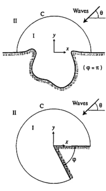
These model equations are capable of simulating wave

refraction, diffraction and reflection for two types of ocean

topography, as shown in Figure 1, i.e.,

t Mac OS is the Macintosh operation system ofApple Computer, Inc.

tt PostScript is a trademark ofAdobe Systems, Inc.

(1} Coastal harbor model (0 < Cp < 71).

(2} Islands model.

Figure l.Two types ofocean topography handled by CATWAVES.

• waves approaching a coastal harbor and

• waves approaching islands in the open ocean.

Additionally, the CATWAVES can handle wave motion in a

region where the discontinuity ofwater depth occurs. Therefore,

the boundary conditions handled in the model are:

• wave reflection along the shorelines and the boundary ofcoastal structures,

• water depth discontinuity, such as step-like changes in

reef coasts, and

• the Sommerfeld radiation condition at infinity.

For linear and nonlinear wave analyses, the numerical method

in terms ofthe infinite element for the exterior region (Tsutsui,

1999,2000) is newly developed to handle the boundary condition

at infinity. As the results, the finite element methodology, in this

case, governs all the regions ofthe problem. The coupling method

(4)

is also applied only to the linear wave analysis.

Note that phenomena of wave breaking of progressive waves

near the shorelines and of standing wave-type breaking in front of the coastal structures are not considered because the decision ofbreaker zones and/or breaking points is at this time very difficult. If possible, the treatment of wave breaking is straightforward (Tsutsui, 1993;Sulaiman,etal., 1994).

2.2 Background to the Numerical Model

The essential requirements for the finite element analysis in CATWAVES are:

• For the harbor model, there must be a straight coastline in the far field, along which the positive x-axis being set up, and the

angle q> formed by die two straight coastlines in the far field is

within the range from 0 to 7C, as shown in Figure 1 (1).

• Therefore, the CATWAVES can handle the unbounded

domain where there exists a semi-infinite breakwater or a wedge-shaped coast, such as results of reclamation.

• All the bathymetric changes must be located near the coordinate origin, as shown in Figure 1 (1).

• For die islands model, similarly, islands must be located near the coordinate origin, as shown in Figure 1 (2).

• The wave field should be divided into two regions - (I) an interior region and (II) an exterior region - by the arc or the circle denoted by C in Figure 1.

• The coastal topography and the water depth must change only in the interior region (I) that is the wave field of the finite element model.

• On the contrary, the water depth in the exterior region (II) is assumed to be constant, where the infinite element is applied and/or die series solution ofthe coupling method is formulated. • Two kinds of the method, therefore, are adopted to impose

the boundary condition at infinity.

(1) The interior and exterior regions are totally dealt widi the finite and infinite elements.

(2) The interior finite element solution and the exterior series solution are coupled on the temporary boundary C.

In appendix, the model equation of wave motion and the

sequence of equations to be solved are described briefly. The user

of CATWAVES is assumed to be familiar with the model equations, such as the mild-slope equation, and the finite element

methodology (Zienkiewicz, et al., 1977,1989). As such, no more explanation of either is included here.

2.3 Model Structure

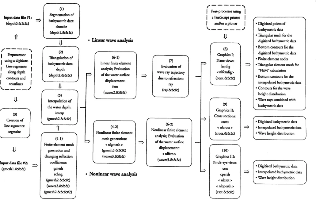
The structure of CATWAVES is composed of three parts; (I) mesh generation,

(II) finite element solution and (III) graphics routines.

All the programs are coded in Fortran and there is no machine-depended statement/command. The flow of procedures and

input/output (I/O) data files arc shown in Figure 2.

• The user is required to create two kinds of initial data files:

"depthO.&&&" for Routine 1 and "gmesh 1.&&&" for

Routine 4-1, where die characters "&&&" denote the part of the file name defined by die user.

• For this purpose, you should prepare data for line segments along die coastlines and depth contours by using a preprocessor. • The programs coded in Fortran in each routine are defined as the routine name plus "m.f' for the main program and n.f' for the subprogram.

• Since the data files with ".&&&" except for the two initial data files will automatically be created in each routine, use them as the input data files in the succeeding process. • Internal OPEN/CLOSE statements are used for the definition

of I/O data files and hence the logical unit numbers (31,32,

..., 91, 92,...) used in die routines must be fixed.

• The I/O data file names shown in the parentheses, "depthO", "depth 1", "depth2", "gmeshl", ngmesh2", Bgmesh3", "waves2", "waves3", "ray", "cont", "cross" and "cset'Vare

arbitrary but they might be fixed for convenience ofintroducing all the procedures with the aide of an example.

• All the routines work interactively so that you can input necessary data, such as I/O date file names and variables, according to the instructions appearing on the screen. • Considering the problem concerned, however, you should

specify the dimensional parameters that declare the array's dimensional size in the main program.

• Routines necessary for the nonlinear wave analysis are shown in the angle brackets in Figure 2.

(I) Mesh Generation Routine

In order to easily prepare the badiymetric data and create die finite element mesh over the model region, the CATWAVES incorporates with an automatic triangular element mesh generation system (e.g., Lo, 1985).

For the linear wave analysis

• There are two kinds of triangular mesh for bathymetric and finite element regions.

• BauSymetric data are set up on the triangular element mesh by Routines 1 and 2, "damake" and "depuV.

• Routine "segmakc" in (3) creates line segments useful for the mesh generation data file "grneshl.&&£&".

• The triangular finite element mesh for the wave field is

generated by Routine "gmesh" in (4-1).

• If necessary, die reflection coefficients along die shorelines and the boundary of coastal structures can be changed widi the

aide of Routine "rchng" in (4-1).

• The water depth at each triangular element node is linearly

interpolated, by Routine "interp" in (5), from the digitized

badiymetric data already saved in the file "dcpth2.&&&".

For the nonlinear wave analysis

• According to the users request, Routine "gmesh" in (4-1) generates the new file "gmcsh2.&&&#2" that has information

(5)

Input data file #1 (depthO,&&&)

ft

1 1 /**"~ — — —— «> 1 Preprocessor ■ using a digitizer, . Line segments afont* rl^nfh . cuuiig ucpui

' contours and

1 1 coastlines V. J (3) Creation of Itne segments: segmake V J

Input data file #2: (gmeshl.&&&) (1) Segmentation of bathymetric data: damake (depthl.&&&)

u

r s \ ₍₂₎ Triangulation of bathymetric data: depth (depth2.&&&)

1 U

(5) Interpolation of the water depth:

interp (gmesh2.&&&)

—s -—•

(4-1) Finite element mesh

generation and changing reflection coefficients: gmesh rchng (gmesh2.&&&) (waves2.&&&) (gmesh2.&&&#2)

J

linear wave analysis

Linear finite element analysis; Evaluation

ofthe water surface displacement:

fern

(waves2.&&&)

(4-2)

Nonlinear finite element mesh generation:

< nlgmesh >

(gmesh3.&&&)

(waves3.&&&:)

Noninear wave analysis

(7)

Evaluation of wave ray trajectory

due to refraction:

ray

(6-2)

Nonlinear finite element analysis; Evaluation ofthe water surface

u

(8) Graphics I; Plane views: femfig <nlfemfig> (cont.&&&) (9) Graphics II; Cross sections: cross < nlcross > (cross.&&&) (10) Graphics III; Bird's-eye views: cset cperth < nlcset > < nlcperth > • Digitized points of bathymetric data

• Triangular mesh for the digitized bathymetric data

• Bottom contours for the digitized bathymetric data • Finite element nodes • Triangular element mesh for

"FEMM calculation • Bottom contours for die

interpolated bathymetric data • Contours for the wave

height distribution • Wave rays combined with

bathymetric data

Digitized bathymetric data Interpolated bathymetric data

Wave height distribution

Digitized bathymetric data Interpolated bathymetric data Wave height distribution

(I) Mesh generation and 00 Finite element solution routines.

Figure 2. Structure of CATWAVES.

(6)

of the generated linear element mesh and is used to create the

nonlinear finite element mesh.

• This is Routine "nlgmesh" in (4.2) that generates the 6-nodes triangular element mesh in the specified region for the nonlinear

wave analysis.

(II) Finite Element Solution Routine

There are two main routines for the wave analysis:

• Routines "fem" and "nlfem" in (6) for linear and nonlinear

wave analyse are the main components of CATWAVES and

evaluate the water surface displacement at all the nodes of

triangular mesh.

• Based on the digitized bathymetry, Routine "ray" in (7) evaluates the wave ray trajectory due to refraction, the results ofwhich can be combined with bathymetric data in graphics routines.

(III) Graphics Routine

In order to visualize all the numerical results, vector data both for bathymetry and the wave height are generated with the post

processors, Routines 8,9 and 10. The routines with "nl" in their

names are for the numerical results ofthe nonlinear wave analysis. • For plane views, Routines "femfig" and "nlfemfig" in (8)

generate vector data describing the digitized points, finite

element nodes, triangular element mesh, contours for bathy

metry and wave height distribution, and wave rays. • Data for the cross section ofbathymetry and wave height distri

bution are created by Routines "cross" and "nlcross" in (9). • Routines "cset", "cperth", "nlcset" and "nlcperth" in (10) are

for getting bird's-eye views (perspective projection).

There are two kinds of vector data generated by the graphics routines 8 and 10.

• The first data are for convenience of providing for a plotting routine. A viewer for graphics, CATFIG, is presented. This is written in the C-language and works with Mac OS. • The second data are written in the PostScript language, which

should be handled by commercial-base graphics software and produce hi-qualicy graphics.

3. General Rules for Mesh Generation 3.1 Overview

Since the system of triangular element mesh generation plays

a significant role in handling bathymetric data and finite element grids, the general rules behind mesh generation is described. With the aide of segmentation of coastlines and depth contours, the finite element mesh in CATWAVES consists ofthe typical five line segments, including three particular mesh patterns, and the

central mesh.

3.2 Segmentation Processes

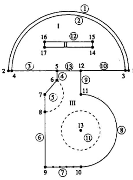
1. Divide, in general, the bathymetry and the wave field of the

finite element model into several subregions by line segments,

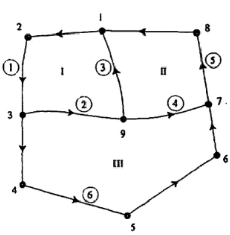
as shown in Figure 3. This process is normally essential because

Figure 3. Division of the wave field into three subregions.

of the following reasons. For bathymetric data

• In digitizing bathymetry, the data spacing depends on the density ofdepth contours and, therefore, you should digitize the shorelines and depth contours so as to get their smooth lines in graphics.

For the finite element mesh

• The computational accuracy of the water surface displace ment is directly affected by the element mesh size that must be decided according to the local wave length. For example, the mesh size recommended is about 1/15-1/20 ofthe local wave length. Therefore, you should vary the element mesh size locally.

• Dividing the wave field such that there are nearly the same number ofnodes in each subregion, you can save computing time.

2. The line segments are specified by the beginning and ending nodes, defined by the intersection of these line segments and by additional nodes.

3. Number all the nodes, line segments and subregions. For example, in Figure 3, the wave field is divided into three

subregions (I, II and III) by six line segments, (l)-(6), with

the beginning and ending nodes 1,3,7 and 9. Notes:

• The important premise in the numbering of nodes is that the nodes along line segments for the exterior boundary should be numbered anti-clockwise. For example, the line

segment (1) is defined by the nodes 1-2-3.

• This means that, by following the boundary line segment, the particular subregion ofinterest, e.g., the region I in Figure

3, is always on the left-hand side.

• An exception to this rule is numbering of nodes on the

interior common line segments for the subregions, i.e., (2),

(3) and (4) in Figure 3. Since unidirectional numbering both

for the right and left subregions is impossible, the direction

of numbering is arbitrary only in this case.

4. Define each subregion as a region surrounded by a set ofthese

line segments. It is important that me first line segment be a line on which the nodes are numbered anti-clockwiseaccording

(7)

14 TSUTSUI: CATWAVES, Prediction of Linear and Nonlinear Wave Motion in Unbounded Coastal Domains

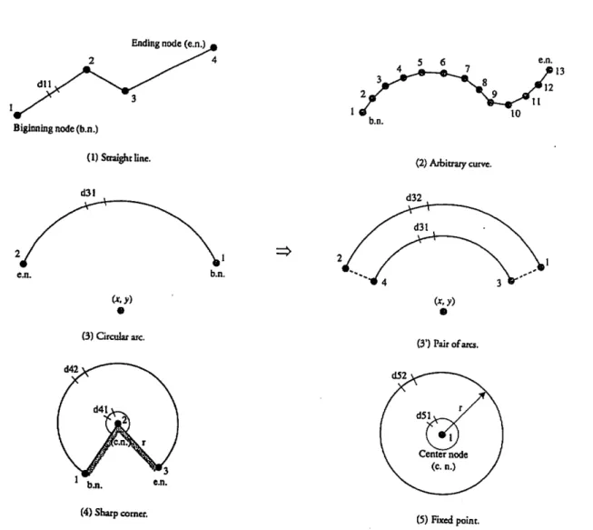
Table 1. Five types of line segments and data structure.

Types Index (is) Data structure etc. (See Figure 4)

Straight line Arbitrary curve Circular arc Sharp corner Fixed point 1* 2* 3* 4" 5*

Beginning and ending nodes, (if necessary, intermediate nodes), spacing on a line. Beginning, intermediate and ending nodes.

Beginning and ending nodes, center coordinate, spacing on an arc.

(A pair ofarcs is made by two arcs between which the mesh is generated, as shown in Figure 5.)

Beginning, center and ending nodes, radius of an outer arc, spacing on an inner and outer arcs.

CFhe refine mesh is progressively generated around a sharp corner, as shown in Figure 6.) Center node, radius of an outer circle, spacing on an inner and outer arcs.

(The radiarory mesh is generated from a fixed point, as shown in Figure 7.)

Ending node (e.n.)

dll Biginningnode(b.n.) (1) Straight line. ix.y) (3) Circular arc. d42 (5) Fixed point.

. Five types ofline segments used in the finite clement mesh generation routine.

to thepremise3 above. For example, ifthe nodes are numbered

in the direction ofthe arrows in Figure 3, the subregion II

should be defined as (4)-(5)-(3) or (5)-(3)-(4).

5. Ifbathymetric discontinuity exists, such as step-like disconti

nuity ofthe waterdepth, you should divide the wave field into

subregions by the line segments along discontinuity and

number the subregions from deeper to shallower ones.

3.3 Five Types ofLine Segments

(8)

Figure 5. Pair of arcs between which the mesh is

generated.

Figure 6. Mesh generation around a sharp coner. Figure 7. Mesh generation about a fixed point.

Figure 4, are used in the finite elemenc mesh generation routine. The index "is", a two-digit integer number, is used to define the type and the physical characteristic of each line segment. The type ofa line segment is classified by the number from 1 to 5t as defined in Table 1. The first row of "is", * inTable 1, is an indicator specifying the physical characteristic of a line segment. The following rules are defined:

1. Straight lines, arbitrary curves, circular arcs and sharp corners (in Figure 4 (4), lines 1-2-3 only) may be real boundaries, such as coasdines. In this case, let the first row ofindex "is" be "0" and specify the reflection coefficient along them. 2. If bathymetric discontinuity exists, let the first row of index

"is" be "1".

3. For the other cases, the first row should be a number except for "0"and"l".

4. The spacing, dl 1, d31,.... is used to decide the additional intermediate nodes on each line segment.

3.4 Three Kinds of Particular Mesh

Figures 5-7 show particular mesh generated between a pair of arcs, around a sharp corner and about a fixed point.

3.5 Central Mesh Generation

In the central subregion except for three kinds of particular mesh given in Figures 5-7, the equilateral triangular mesh is

generated as much as possible. The reason is that, in the finite

element analysis, the numerical error for the equilateral triangular

element is the minimum among those for all types oftriangles

with the same size.

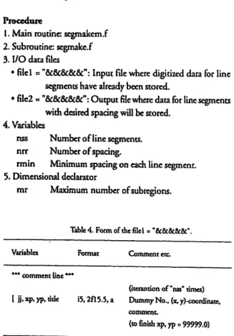
4. Procedures in CATWAVES 4.1 Overview

The best way to understand how to use CATWAVES is to

examine it with the aide ofan example. This chapter is intended

to introduce all the procedures according to Figure 2, and describe

the I/O data files, variables, dimensional declarators and the data

form in each routine.

The frame for introducing each routine in CATWAVES is as

follows:

1. Main routine: Name of the main program.

2. Subroutine: Name of the subprogram.

3. I/O data files: Name of I/O data files and their concents.

4. Variable: Name ofvariables in the routine.

5. Dimensional declarators: Dimensional size of the array and its meaning.

The user of CATWAVES should specify the I/O date files and, if necessary, the variables according to the instructions appearing on the screen. The dimensional declarator should be defined by the PARAMETER statement in the main program. The termination with error messages will be caused when the dimensional space is not enough. In all the routines the spacial and time units are meter and second, respectively.

4.2 Procedures

■ Routine 1: Segmentation ofBathymetric Data

Purpose

This process is preparation for setting up the bathymetric data and therefore collects raw bathymetric data for each subregion, along the shorelines and depth contours.

Segmentation Processes

You have to digitized bathymetric data along the shorelines and depth contours in the following way:

1. Divide the wave field into several subregions.

2. Number all nodes. At this point, the nodes are intersections of

line segments and other necessary points. 3. Number all lbe segments and subregions. 4. Define line segments.

5. Define subregions by a set ofthese line segments.

6. Digitize depth data on line segments with suitable spacing. 7. Digitize interior depth data in each subregion with spacing

suitable for interpolation of depth contours.

8. Save data for line segments and subregions in "filer and save

interior depth data in "pfile", according to the bathymetric data form, defined in Tables 2 and 3.

Procedure

(9)

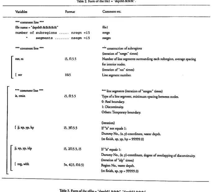
16 TSUTSUI: CATWAVES, Prediction of Linear and Nonlinear Wave Motion in Unbounded Coastal Domains Table 2. Form of thefilel = "depthO.&&&"

Variables

*** comment line **• File name = "depthO.&&&&&H number of subregions . " segments ... Format .... nregn =i5 =i5 Comment ecc. filel nregn nsegm " comment line' ass, sz [ ntr i5,fl5.5 10i5 *** construction ofsubregions

(iteration of "nregn" times}

Number of line segments surrounding each subregion, average spacing

for interior nodes. (iteration of "nss" times)

Line segment number.

**• comment line'

is, rmin i5. fl5.5

*** line segments (iteration of "nsegm" times)

Type ofa line segment, minimum spacing between nodes.

0: Real boundary. 1: Discontinuity.

Others: Temporary boundary.

jj, xp, yp, idp [ nrg,whh 15, 3fl5.5 i5,2fl5.5,i5 5x, 4(i5. fl0.5) (iteration) If "is" not equals 1:

Dummy No., (x, y)-coordinatc, water depth, (to finish, xp, yp, hp = 99999.0)

If "is" equals 1:

Dummy No., (x, y)-coordinate, degree ofoverlapping ofdiscontinuity,

(iteration of "idp" times) Region No., water depth,

(to finish, xp, yp = 99999.0)

Table 3. Form of the pfiles = "depth01.&&&", "depthO2.&&&"

Variables *** comment line' *** comment line' [ xp,yp,hp Format 5x,3fl5.5 Comment etc. (iteration)

(x, y)-coordinare, water depth.

(to finish, xp, yp, hp •» 99999.0)

2. Subroutine damakef

3. I/O data files

•fiiel = "depthO.&&&": Input file where data for line

segments and subregions have already been stored.

• pfile . "depth01.&&&", "depthO2.&&&",.... Input Hle(s)

where digitized interior bathjrmetric data in each

subregion have already- been stored.

• file2 = "depthl.&&&": Output filewhere the digitizedpoints

ofbathymetric data will be stored.

4. Variable

nfend Number ofpfile(s).

5. Dimensional declarators

mr

Maximum number ofsubregions.

ms Maximum number of line segments, mn 1 Maximum number of boundary nodes.

mn2

Maximum number of interior nodes in each

sub-region.

Since, in general, interior depth data along the depth contour

lines and necessary points could be stored separately in some

files, this routine ask the user to input the number of"pfiles" and

(10)

The forms of input data files are defined in Tables 2 and 3. Notice that:

• The bracket means the range of iteration and the iteration count is in the comment column.

• The line segments surrounding each subregion must be closed. • For the bathymetric data, the type of line segments is an arbitrary line, hence the index "is" is a single-digit integer number, i.e., "0"," I",..., only to define physical characteristics (Refer to 3.3).

• Data on line segments are selected by checking whether the distance of adjacent nodes is greater than "rmin".

• For a bathymetric point necessary for segmentation, set the dummy number jj be "99999" and therefore the point is selected even if the distance is less than "rmin".

• Similarly, interior points for each subregion are selected accord ing to the spacing "sz". This routine excludes the unnecessary points that do not belong to any subregion.

B Routine 2: Triangulation of Bathymetric Data

Purpose

This routine generates the triangular mesh for digitized bathymetric nodes. Details of bathymetry are finally furnished

on the set of triangular elements. Procedure

1. Main routine: depthm.f 2. Subroutine: depth.f 3. I/O data files

• filel = "depthl .&&&": Input file where the digitized points ofbathymetric data have already been stored. • file2 = "deprh2.Sc&&": Output file where, after triangulation,

details of bathymetric data will be stored.

Maximum number ofsubregions. Maximum number ofline segments. Maximum number ofelements.

Maximum number of nodes.

Maximum number of boundary nodes.

Maximum number of interior nodes in each

sub-Waves mr ms mn mnl mn2 region.

Example of a Harbor Model

Here, consider an example ofan artificial harbor model with a

submerged breakwater in front ofthe harbor mouth, as shown in

Figure 8 (1). In the semicircular region ofthe harbor, the water

depth decreases uniformly from 20m to 10m, as shown in the

cross section A-A. There is discontinuity along the submerged

breakwater where the water depth changes abrupdy from 20m

to 10m. Forsimplicity, let thewater depth in the remainingregion

be constant, say, 20m. It is assumed that there is the vertical wall

along the shorelines. The reflection coefficients along shorelines,

as shown in Figure 8 (1), are assumed to be 1.0, 0.5 and 0.3.

Figure 8 (2) shows the coordinate system and the shape

ofcoast-20.0m Submerged ,-breakwater "" 1.0 hd = 10.0m (1) Artificial harbour.

(2) Coordinate system and bathymetry.

(3) Segmentation ofbathymetric data. Figure 8. An artificial harbor model.

(11)

18

TSUTSUI : CATWAVES, Prediction of Linear and Nonlinear Wave Motion in Unbounded Coastal Domains

lines for bathymetry that covers the harbor model to interpolate

the nodal water depth.

The bathymetry is divided into three subregions, as shown in Figure 8 (3):

(I) the offshore region,

(II) the region on the submerged breakwater and (III) the region in the harbor.

The nodes and line segments are set up. The cross in all the subregions denotes internal points thatassumed to be on the depth contour lines. Notice that, in this example, the wave field on the

submerged breakwater is subdivided along the depth discontinu ous line (6).

■ Routine 3: Creation of line Segments

Purpose

This routine creates line segments (straight and arbitrary lines) with desired spacing. The results can be used in the input data file, "gmcshl.&&&", for finite element mesh generation. Notes that:

• You have to use the coastlines and particular depth contour tines with suitable spacing as the line segments for finite element mesh generation.

♦ The graphics routine "cross" helps you to generate raw bachymetric data useful for this purpose (Refer to Notes in Routine 9: Graphics II- Cross Sections).

Procedure

1. Main routine: segmakem.f 2. Subroutine: scgmake.f 3. I/O data files

• file1 = "6:8c&&6c": Input file where digitized data for line

segments have already been stored.

• filc2 = "&&&&&": Output file where data for line segments

with desired spacing will be stored. 4. Variables

nss Number ofline segments.

nrr Number ofspacing.

rmin Minimum spacing on each line segment. 5. Dimensional declarator

mr Maximum number ofsubregions.

Table 4. Form ofthe filet = "&&&&&".

Variables Format Comment etc

••* comment line ***

(iteiantion of "nss* times)

I jj. xp, yp, tide i5.2H5.5, a Dummy No., (x. y)-coo«linate,

comment.

(to finish xp,yp = 99999.0)

The form ofinput data for creation ofline segments is defined in Table 4. The bracket means the range of iteration and the

iteration count is in the comment column.

■ Routine 4: Finite Element Mesh Generation and Changing Reflection Coefficients

Purpose

The procedure presents two kinds of routine for generating the linear and nonlinear finite element mesh and also the routine for changing reflection coefficients along the shorelines and the boundary ofcoastal structures.

(1) Finite Element Mesh Generation

This routine generates the triangular element mesh over the wave field of the finite element model and provides you with capabilities of:

(a) changing the element mesh size in each subregion and (b) making the variable-band width ofthe coefficient matrix

of the system oflinear equations small. Remark that:

• The first demand (a) is realistic and, to do so, the wave field must be divided into subregions.

• The second one (b) comes from computational problems. Since the coefficient matrix of the system is sparse, the smaller the variable-band width of the coefficient matrix, saves the computer storage and, as a result, computing time. This task is accomplished by the procedure: renumbering ofnode numbers included in CATWAVES.

• The algorithm of renumbering of node numbers is similar to a widely-used Cuthill & McKee (1969) ordering, to reduce the variable-band width.

• Details of the generated finite element mesh are prepared for interpolation of the nodal water depth in Routine 5. Segmentation Processes

As described in Chapter 3: GeneralRulesfir Mesh Generation, the segmentation processes for finite element mesh generation

are:

1. Divide the wave field into several subregions.

2. Number all nodes. At this point, the nodes are intersections of

line segments and other necessary points.

3. Number all line segments and subregions.

4. Define line segments.

5. Define subregions by a set of these line segments. 6. Decide spacing on line segments.

7. Decide elements mesh sizes required for subregions. 8. After preparation, save data in "filel", according to the data

form ofthe finite element mesh, defined in Table 5. Reflection Coefficients

Among the five line segments, straight lines, arbitrary curves,

circular arcs and sharp corners may be boundaries along which

(12)

you have to specify reflection coefficients, according co the

following rules:

1. Reflection coefficients at all boundary nodes should be given

in advance.

2. Intermediate nodes are automatically created for straight lines,

circular arcs and sharp corners.

3. Reflection coefficients at these additional nodes on the

boundaries are evaluated as the same value ofthe former node,

e.g., in Figure 4, • for a straight line:

the value at the node 1 along the line 1-2, the value at the node 2 along the line 2-3, die value at die node 3 along the line 3-4, • for a circular arc the value at the node 1, • for a sharp corner: the value at the node 2.

4. For arbitrary curves, you should input reflection coefficients at

all the nodes. However, ifsome of the reflection coefficients

are successively the same, it is enough co input the value only

at the beginning node (Refer to Table 5). (4.1) Procedure for linear Mesh Generation

1. Main routine: gmeshm.f 2. Subroutine: gmesh.f 3. I/O data files

• filel »Mgmeshl.&&&": Input file where data for line segments and subregions have already been stored.

• file2 = "gmesh2.&&&": Output file where details of the

generated linear element mesh will be stored.

• file3 = "waves2.&&&": Output file where details of the

reflection coefficient will be stored.

• file4 »"gmesh2.&&&#2": Output file where detail informa tion of the generated linear element mesh will be stored. This file will be created according to the user's request to generate nonlinear finite element mesh. 4. Variables

hO Constant water depth in the exterior region (in meters),

irenum Parameter for renumbering of node numbers; 0: No renumbering.

1: Renumbering to reduce the variable-band width of the coefficient matrix of the linear system, imesh Parameter for output the file4 = "gmesh2.&&&#2";

0: No output (default). 1: Output.

ms Maximum number ofline segments.

mm Maximum number ofelements.

mn Maximum number of nodes.

mnl Maximum number ofboundary nodes.

mn2 Maximum number of interior nodes in each

sub-region.

mk

Maximum number of nodes on straight lines and

curves.

mi

Maximum number of layers in the three kinds of

particularly generated mesh, i.e., a pair ofarcs, a

sharp corner and a fixed point.

The form of input data for finite element mesh generation is

defined in Table 5. Noce that:

• The bracket means the range of iteration and the iteration

count is in the comment column.

• Exclude the number ofsubregions defined by "pair ofarcs",

"sharp corner" and "fixed point" from the input number of

subregions, "nsubr".

• Similarly, exclude the number of nodes on arbitrary curves

from the input numbers of nodes, "ninpt", "nbinpt" and

"ndinpt".

• In order to satisfy the assumption in Chapter I: Background andStructure for the finite element method, the outer segment mat separates the interior region from the exterior region should

be:

(1) a semi-ring for a harbor model or a ring for an islands

model, and

(2) the first line segment should be an arc or a circle. • To obtain a circle; let the beginning and ending nodes ofan

arc be the same node.

• The line segments surrounding each subregion must be dosed. (4.2) Procedure for Nonlinear Mesh Generation

Before running this routine, the user should prepare the mesh

and wave data files, i.e., "gmesh2.&&&", l1waves2.&&&" and

"gmesh2.&&&#2", by the linear mesh generation routine "gmesh" in (4-1) and interpolate the nodal water depth in terms of Routine "interp" in (5).

1. Main routine: nlgmeshm.f 2. Subroutine: nlgmesh.f 3. I/O data files

• filel ="gmesh2.&&&": Input file where details of the generated linear element mesh and die nodal water depth have already been stored.

• file2 = "gmesh2.&&&#2": Input file where detail information of the generated linear element mesh have already been stored.

• file3 = "waves2.&&&": Input file where details of the reflection coefficient for the linear wave analysis have already been stored.

• file4 = "gmesh3.&&&": Output file where details of the generated element mesh and the nodal water depth

for die nonlinear wave analysis will be stored. • file5 = "waves3.5c&&": Output file where details of the

reflection coefficient for the nonlinear wave analysis will be stored.

4. Variables

he Critical water depth (in meters); the region with the water depdi shallower than this value is assumed to be the region ofthe nonlinear wave analysis.

(13)

20 TSUTSUI: CATWAVES. Prediction of Linear and Nonlinear Wave Motion in Unbounded Coastal Domains

Table 5. Form of the filel = "gmeshl.&&&".

Variables Format Comment etc.

**• comment line ***

file name = "gmesh 1 .&&&&&" file 1

number of subregions nsubr =i5 nsubr

* input nodes ninpt =i5 ninpt

" input boundary nodes nbinpt =i5 nbinpt

* input discontinuity nodes . . ndinpt =i5 ndinpt

" segments nsegm =i5 nsegm

* pairs of arcs nparc =i5 nparc

" sharp corners nscor =i5 nscor

* fixed points nfpts =i5 nfpts

*** comment line "** (iteration of "ninpt" times)

I jj, wx, wy i5,2fl 5.5 Dummy No., (x, y)-coordinatc.

*** comment line If nbinpt > 0: (iteration of "nbinpt" times)

{ jj, ibw.wrc 2i5, ft0.5 Dummy No., boundary node, reflection coefficient.

•** comment line *** Ifndinpt > 0: (iteration of "ndinpt" times)

I jj» idw 2i5 Dummy No., discontinuity node.

•** comment line "* [f nparc > 0: (iteration of "nparc" times)

[ kpaicl, kparc2 2i5 Line segment numbers ofa pair ofarcs.

•M comment line — «• construction ofsubregions

(iteration of "nsubr" times)

nss'sz i5,fl5.5 Number ofline segments surrounding each subregion,

element mesh size. (iteration of "nss" times)

* ntr t0i5 Line segment number.

*'* line segments (iteration of "nsegm" times)

"•(DstraightUnes- ~ comment line

*5 Type ofa line segment.

nel'dl l

'5. fl0.5

Number ofnodes, spacing on a line.

(iteration of "nel" times)

1 ndl

10.5 Node number.

•" (2) arbitrary curves ••• ... commem ^

'5 Type ofa line segment.

nd21 ;e₁₇ d • •_{Beginning node.}i

(iteration)

I M. xp. yp. re i5i 3fl5 5 Dummjr ^^ fc y).coordinate) (£f neccssaiy> ^^

(to finish, xp, yp = 99999.0)

'5 Ending node.

*** (3) circular ares'" ..._{comment line}..

, , '* Type ofa line segment.

nd31tnd32,x30,y30,d31 2i5 ?fin s_w,nw.j r • •_{Beginning and ending nodes, center coordinate, spacing on an arc.}j j. .

•-(4) sharp corners ••• ... ..

comment line

15 ._

... ,., ,_ l5 Type of a line segment

nd41,nd42.nd43.r4.d4l,d42 3i5 3nos_{jo. atiw.j} n • •_{Beginning, center and ending nodes, radius of an outer arc,}. , spacing on an inner and outer arcs.

*"• (5) fixed points —

comment line

Hl5.Ad51.d52

lm,

Typeofa.inesegment.

w 3HV3 center node, radim ofan outer circle, spacing on an inner and outer circles.

(14)

mm Maximum number ofelements,

mn Maximum number ofnodes,

mn 1 Maximum number ofboundary nodes.

mn2 Maximum number of interior nodes in each

sub-region.

(2) Changing Reflection Coefficients Along Boundaries After generation of the finite element mesh, Routine "rchng" in (4-1) can change the reflection coefficients along the shorelines and the boundary of the coastal structures. Notice however that to modify the reflection coefficients in the file "waves3.Bc&&"

for nonlinear wave analysis, you should make new file "waves2. &&&" by using this routine and later create the nonlinear finite

element mesh with the aide of Routine "nlgmesh" in (4-2). Procedure

1. Main routine: rchngm.f

2. Subroutine: rchng.f 3. I/O data files

• filel = "gmeshl.&&&": Input file where data for line segments and subregions have already been stored. New reflection coefficients to be modified should be

specified in this file.

• file2 a "gmesh2.&&&": Input file where details of the generated linear element mesh have already been

stored.

• file3 = "waves2.&&&": Input file where details of the

reflection coefficient have already been stored.

• file4 = "waves2.&&&": Output file where details of the modified reflection coefficient will now be stored.

ms Maximum number of line segments.

mn 1 Maximum number of boundary nodes.

mn2

Maximum number of interior nodes in each

sub-mk

region.

Maximum number of nodes on straight lines and

curves.

Note that data for new nodal reflection coefficients desired

should be specified in "filel" and the modified reflection coeffi

cients will be stored in the new file "file4". Example of the Harbor Model

Consider the artificial harbor model, as was shown in Figure 8

(I). Figure 9 shows the result ofsegmentation of the wave field;

the nodes, line segments and subregions being numbered.

According to the fourth note in Procedurefor Linear Mesh

Generation, the outer region is the semi-ring defined by a pair of

arcs. To illustrate all line segments defined in CATWAVES, there

is an arbitrary curve between the nodes 9 and 10, a sharp corner

along the shoreline 6-7-8, and a fixed point about the node 13.

10

Figure 9. Segmentation of the wave field.

The others are straight lines.

As was seen in Figure 8 (1), the reflection coefficients are assumed to be:

1.0 along lines 2-4-5 and 1-3-12,

0.5 along lines 5-6-7-8-9-10 and 11-12, and

0.3 along the arc 10-11.

Note that the shape ofthe subregion on the submerged breakwater divided by the depth discontinuous line (12) is identical with die

corresponding region of bathymetry in Figure 8 (3).

B Routine 5: Interpolation ofthe Water Depth Purpose

So far, the bathymetric data file "depth2.&&&" and the finite

element mesh data file tfgmesh2.&&&" have been created.

Referring to the bathymetric data, diis routine completes the mesh

data by linearly interpolating the nodal water depth.

Procedure

1. Main routine: interpm.f 2. Subroutine: interp.f

3. I/O data files

• filel o "depth2.&&&": Input file where, after triangulation,

details ofbathymetric data have already been stored.

• file2 = Mgmesh2.&&&": Input/output file where details of

the generated linear clement mesh have already been

stored. After interpolation, the nodal water depth will

be added. 4. Dimensional declarators

mm Maximum number of elements,

mn Maximum number of nodes,

(15)

22 TSUTSU1 : CATWAVES, Prediction of Linear and Nonlinear Wave Motion in Unbounded Coastal Domains ■ Routine 6: Finite Element Analysis - Evaluation of Water

Surface Displacement -Purpose

This routine evaluates the water surface displacement at all the finite clement nodes based on the finite clement method in

terms of the infinite clement (Tsutsui, 1999, 2000) and the

coupling method (Chen and Mei, 1975; Mei, 1983). (6.1) Procedure for the Linear Wave Analysis 1. Main routine: fcmm.f

2. Subroutine: fcm.f 3. I/O data files

• filcl - "gmcsh2.&&&": Input file where details of the generated linear clement mesh and the nodal water depth have already been stored.

• fllc2 = "wavcs2.&&&": Input/output file where details of the reflection coefficient have already been stored. After calculation, the water surface displacement at all the nodes will be added.

4. Variables

T Wave period (in seconds).

thi Incident angle ofwaves (in degrees), measured anti clockwise from die positive x-axis, as in figure 1. 5. Dimensional declarators

mr Maximum number of subregions.

mm Maximum number of elements.

mn Maximum number ofnodes.

mnl Maximum number of boundary nodes.

mn2 Maximum number of nodes on the exterior arc or the exterior circle; This value is an index to the variable-band width of the sparse coefficient matrix of the linear system.

mn3 Maximum number of nonzero elements in the coefficient matrix of the linear system; Since the coefficient matrix is sparse and symmetric, nonzero elements in the right-upper triangular matrix arc stored in the one-dimensional array. An estimated value ofmn3 is about 0.01 Xmn(mn+l)/2. 6. Solution of the sparse linear systems

Since, in the linear wave analysis, the coefficient matrix ofthe system oflinear algebraic equations is ofsparse and symmetric, the so-called skyline method is implemented to solve the system.

The numerical results of the water surface displacement,

normalized by die incident wave amplitude, are complex values and the wave profile is sinusoidal. So that the nodal wave height

relative to die incident wave amplitude is evaluated by taking the absolute value of the water surface displacement.

(6.2) Procedure for the NonlinearWave Analysis

1. Main routine: nlfemm.f 2. Subroutine: nlfem.f 3. I/O data files

• filel = "gmesh3.&&&": Input file where details of the

generated nonlinear element mesh and the nodal water depth have already been stored.

• file2 = "waves3.&&&": Input/output file where details of the reflection coefficient have already been stored. After nonlinear evaluation, the water surface displacement at all the nodes will be added.

4. Variables

T Wave period (in seconds),

thi Incident angle ofwaves (in degrees), measured anti clockwise from the positive x-axis, as in Figure 1.

nf Number of Fourier modes.

aO Offshore incident wave amplitude (in meters). 5. Dimensional declarators

mnf Maximum number of Fourier modes.

mm Maximum number of elements.

mn 1 Maximum number of boundary nodes.

mn2 Maximum number of nodes on die exterior arc or the exterior circle.

mn3 Maximum number of nonzero elements in the coefficient matrix of the linear system; An estima ted value of mn3 is about 0.02X mn(mn+l)/2. mn4 Maximum number ofunknowns in the final coupled

system (= mnf Xmn)

mn5 Maximum number of nonzero elements in the coefficient matrix ofthe final coupled system (= mnf Xmnfxmn3)

mn6 Maximum dimensional size of the one-dimensional array where all the values of entries (fill-in) in the process ofGaussian elimination are stored. Note that the required space, mn6, for LU decomposition is a few times the number of nonzero elements, mn5-6. Solution of the sparse nonlinear systems

The model equation for nonlinear waves leads, after quasi-lincarization of die nonlinear terms, to the system of nonlinear algebraic equations, i.e., the unknown water surface displacement appears in the coefficient matrix of die system. The system is the coupled system of Fourier components specified and then the coefficient matrix is sparse, large and numerically unsymmetric but has the symmetric structure.

There may be some methodologies for solving this nonlinear system. Typical methods are (1) the direct iteration and (2) the numerical integration of the system ofordinary differential equa tions derived from the original system, in the manner similar to

die incremental method in the structural analysis (Zienkiewicz, et al., 1989) (See Appendix). To the method (1), the simple itera tive method and the Newton method are available. To die mediod (2), on the contrary, die predictor-corrector method, the backward Eulcr method and the Runge-Kutta-type mediod arc available. In all the cases, however, we should solve die unsymmetric system

of linear equations with the parameter of the incident wave

(16)

There exists a number of popular and powerful iterative

methods for solving linear systems, e.g., GMRES (Saad, el. al.,

1986), CGS (Sonnevdd, 1989) and Bi-CGSTAB (van dcrVorst!

1992; Tsucsui, et al., 1998c). The numerical values of the coeffi

cient matrix, however, are of complex due to the boundary

conditions imposed at infinity and therefore suitable precondi

tioned for the methods above and convergence properties are

unknown.

In this package, therefore, the direct methods for sparse matrices

in terms ofsparse matrix techniques (Doff, et al., 1986) are worth

implementing for the key to solution. Among the public domain

software, Howell code MA28 (Duff, 1979) and/or the Y12M

(Zlatev, et al., 1981) are recommend to solve the system ofsparse unsymmetric linear equations. These are written in Fortran and available from netlib*, although the users obtaining MA28 in this way are still requested to sign a license agreement.

Similar to the linear wave analysis, the numerical results of the water surface displacement, normalized by the incident wave amplitude, are complex values. However, the wave profile is not sinusoidal so that, after calculating the wave profile base on the

definition (See Appendix), the nodal wave height is evaluated as

the height between the maximum wave crest and the minimum

wave trough.

Notice that the routine for the nonlinear wave analysis,

"nlfemm", covers the linear wave analysis, too, and therefore the

user can work with this routine both for linear and nonlinear wave motion.

B Routine 7: Evaluation of Wave Ray Trajectory due to

Refraction Purpose

By using the digitized bathymetric data, this routine generates line segments ofthe wave ray trajectory due to refraction. In order

to visualize them combining with bathymetric data, you can use

the graphics routine 8: Graphics I - Plane Views.

Procedure

1. Main routine: raym.f 2. Subroutine: ray.f 3. I/O data files

• file 1 = "depth2.&&&:": Input file where, after triangulation, details of bathymetric data have already been stored. • file2 = "ray.&&&": Output file where data for line segments

of wave ray trajectory will be stored. 4. Variables

hO Constant water depth in the exterior region (in meters).

t netlib is the site of distribution of mathematical software via electronic mail in the Bell Research Labs.

T

Wave period (in seconds).

thi

Incident angle ofwaves, measured anti-clockwise

from the positive x-axis (in degrees),

nray Number ofwave rays,

xr, yr Starting points ofthe wave rays in (x, y)-coordinate

(in meters). 5. Attribute file for variables

• Attribute file = "&&&&&": Input file where all the variables

have already been stored. 6. Dimensional declarators

mm Maximum number of elements,

mn Maximum number ofnodes.

ran 1 Maximum number ofboundary nodes. mr3 Maximum number ofwave rays.

Notes:

• Ifyou have not run this routine yet, the attribute file specifying

the variables necessary for computation will not exist. However,

you can interactively input the variables according to the instructions that appear on the screen, and save them in the

specific file.

• The routine traces a wave ray and when the wave reaches to the shoreline, quits computing.

B Routine 8: Graphics I - Plane Views

Purpose

As the post-processor, the graphics routine plots digitized nodes,

finite element nodes, triangular element mesh, contour lines and

wave rays.

Options

For ndata = 1; Digitized bathymetric raw data ("depthl.&&&"): • job b I: Digitized nodes.

For ndata = 2; Digitized bathymetric data ("depth2.&&&"): • job = 2: Triangular mesh.

• job = 3: Depth contours.

For ndata = 3; Interpolated bathymetric data and the wave height ("gmcsh2.&&&" and "wavcs2.&&&"): • job «s 4: Finite element nodes.

• job = 5: Triangular element mesh. • job = 6: Depth contours.

• job = 7: Contours for wave height distribution. Procedure

1. Main routine: fcmfigm.f 2. Subroutine: femfig.f 3. I/O data files (a) For ndata = 1:

• ftlel n "depthl.&&&": Input file where the digitized points of bathymetric data have already been stored. • file4 = "&&&&&": Output file where vector data for figures

(17)

24 TSUTSUI: CATWAVES, Prediction of Linear and Nonlinear Wave Motion in Unbounded Coastal Domains

(b) For ndata = 2:

• filel n "depth2.&&&": Input file where, after triangulation, details ofbathymetric data have already been scored. • file3 => "ray.&&&": Input file where data for line segments

ofwave ray trajectory have already been stored. • fi!c4 = "&&&&&": Output file where vector data for figures

will be stored.

• filc5 = "cont.fic&fic": Output file where line segments for contours will be stored and used for bird's-eye views in Routine tO.

(c) For ndata o 3:

• filcl n. "gmcsh2.&&&": Input file where details of the generated linear element mesh and the nodal water depth have already been scored.

• file2 « "wavcs2.&&&": Input file where the wave data have

already been stored.

• filc3 = "ray.flc8c&": Input file where data for line segments ofwave ray trajectory have already been stored. • file4 ■ "&&&&&": Output file where vector data for figures

will be stored.

• file5 = "cont.&&&": Output file where line segments for

contours will be stored and used for bird's-eye views in Routine 10.

4. Variables • For general use:

ndata Type of input data (1,2 and 3).

job

Option number (1,2,3,..., and 7).

isgn Index for data output of contours;

0: No output (default).

1: Output when the user wish to use the contour lines of the water depth and/or the wave height distribution for birds-eye views.

iray

Index for combining wave ray trajectory due to

refraction with bathymetric data, only for the cases

of ndata » 2, job = 3 and ndata = 3, job = 6;

0: No combining (default). 1: Combining,

ibound 0: No drawing boundaries. 1: Drawing boundaries (default), ilabel 0: No labeling.

1: Labeling (default),

icoord 0: No drawing the coordinate origin.

1: Drawing the coordinate origin (default).

• For the contours:

mch 1

Number ofcontours for the water depth.

mch2

Number ofcontours for the wave height,

hight

Values ofcontours for the water depth (in meters)

and wave height.

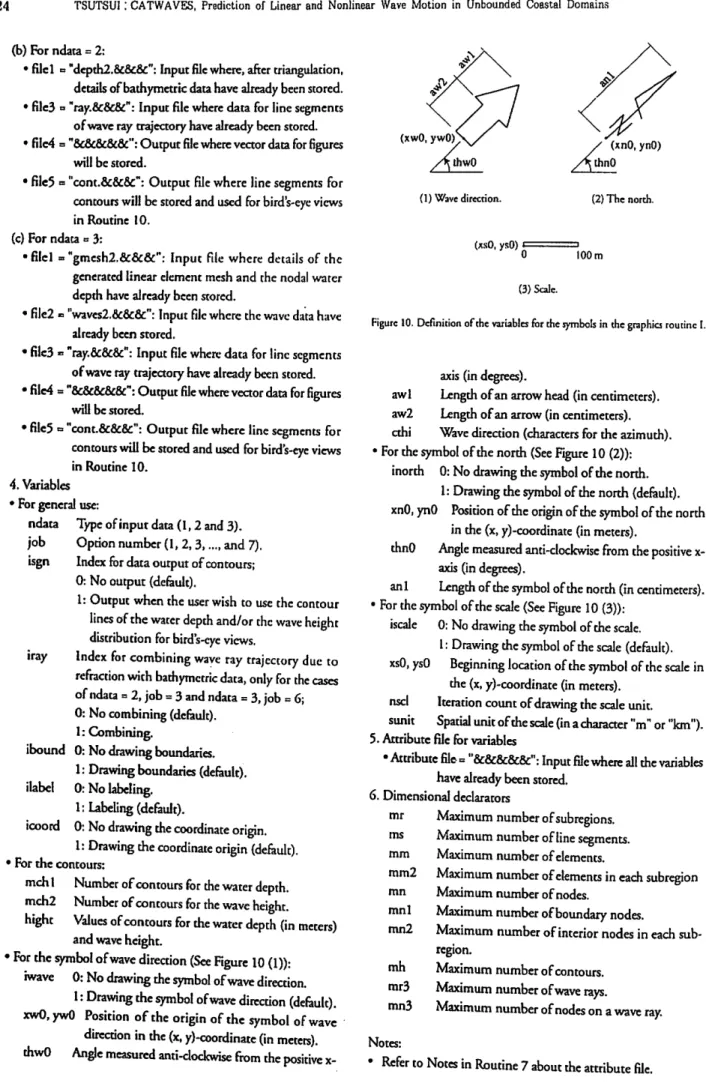
• For the symbol ofwave direction (See Figure 10 (1)):

iwave 0: No drawing the symbol ofwave direction.

1: Drawing the symbol ofwave direction (default).

xwO.ywO Position of the origin of the symbol of wave

direction in the (x, y)-coordinate On meters).

thwO

Angle measured anti-clockwise from the positive

x-(xwO, ywO) / jthwO (1) Wave direction. (xsO, ysO) (2) The north. 0 100 m (3) Scale.

Figure 10. Definition of the variables for the symbols in the graphics routine I.

axis (in degrees).

awl Length ofan arrow head (in centimeters). aw2 Length ofan arrow (in centimeters),

cthi Wave direction (characters for the azimuth).

• For the symbol ofthe north (See Figure 10 (2)):

inorth 0: No drawing the symbol of the north.

1: Drawing the symbol of the north (default). xnO, ynO Position ofthe origin of the symbol ofthe north

in the (x, y)-coordinate (in meters).

thnO

Angle measured anti-clockwise from the positive

x-axis (in degrees),

an 1 Length of the symbol ofthe north (in centimeters). • For the symbol ofthe scale (See Figure 10 (3)):

iscale 0: No drawing the symbol of the scale. 1: Drawing the symbol of the scale (default). xsO, ysO Beginning location of the symbol of the scale in

the (x, y)-coordinate (in meters),

nscl

Iteration count ofdrawing the scale unit,

sunk

Spatial unit ofthe scale (in a character "m" or "km").

5. Attribute file for variables

• Attribute file = "&&&&&": Input file where all the variables

have already been stored.

mr Maximum number ofsubregions. ms Maximum number ofline segments, mm Maximum number ofelements.

mm2

Maximum number ofelements in each subregion

mn Maximum number of nodes,

mnl Maximum number ofboundary nodes.

mn2

Maximum number of interior nodes in each

sub-region.

mh

Maximum number ofcontours.

mr3

Maximum number ofwave rays.

mn3

Maximum number ofnodes on a wave ray.

Notes:

(18)

Table 6. Form of vector data for plane figures.

Variables Format and comment etc.

• Drawing line:

1. lw, Ip T, 2i3

u, xp, yp. d, xp, yp [, d. xp, yp,...] V, 2f7.3. 'd'. 2f7.3 [, •d',2f7.3.

lw: Line width

!p: Line pattern (fixed to be 0 for solid line) (xp, yp): (x, y)-coordinat

"u" denotes pen up and "d", pen down. • Drawing comment and title

c, nc, xp, yp, wh, we, run, rise, slant 'c', i3, 2f7.3, 5f7.2

title

nc: Character size

(xp, yp): (x, y)-coordinate

(wh, we): Height and width ofcharacters (run, rise): (x, y)-vector of incline of the tide slant: Slant of characters

title: Characters

• Ending:

end 'end'

End of data

• The variables for the symbols and their origins shown by ° are defined in Figure 10.

• For the numerical results of the nonlinear wave analysis, use Routine "nlfemfig" and the I/O data files "gmesh3.&&&" and "waves3.&&&". Variables and dimensional declarators and so on are the same with those in Routine "femfig". Form ofVector Data

There are two kinds of vector data generated by this routine: • The first vector data arc for convenience of providing for a plotting routine. The form ofvector data is defined in Table 6. As was noticed before, the bracket means the range ofiteration. • A viewer, CATF1G, is presented for this data. It is written in

the C-language and works with Mac OS.

• The second vector data file, written in the PostScript language, is for commercial-base software that can deal with PS-file. This file is automatically generated and has the characters ".PS" at the end of the vector data file name.

Note that, in the following examples of the three graphics routines, the results for the linear wave analysis are firsdy presented and later the results of the nonlinear wave analysis will be shown.

Examples of Graphics I

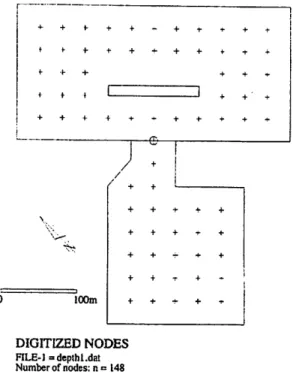
For the artificial harbor model demonstrated before, you can obtain the following graphic results according to the options. • Job = 1: Figure 11 shows the digitized nodes in case of the

100m + + -r + + + + -r + + + * + •* DIGITIZED NODES FILE-1= depthl.dat Number of nodes: n = 148

Figure 11. Disttized points representing bathymetric nodes (job = 1).

/ \

z

\N\i

100m

z

\

A

~ \ DIGITIZED GRIDS OF WATER DEPTH

FILE-1 = depth2.dat Number of elements: m = 225 Number of nodes: n = 143

Figure 12. Triangular mesh generated over the digitized bathymetric data (job = 2).

parameters ibound = 1, ilabel = 1, and icoord = 1. The line segments showing coastlines and temporary boundaries such as along the submerged breakwater are drawn by the solid line

and the interior points, by the cross. The cross with a circle

denotes the coordinate origin. Using this figure, you can check

(19)

26 TSUTSUI '. CATWAVES, Prediction of Linear and Nonlinear Wave Motion in Unbounded Coastal Domains

100m

CONTOURS: WATER DEPTH (Digitized) FILE-l=deplh2.dat

figure 13. Depth contours generated from the bathymerric data (job = 3).

Sharp corner

Fixed point

Figure 15. Three kinds ofparticularly generated mesh in CATWAVES; (1) the pair ofarcs, (2) the sharp corner and (3) the fixed point.

nfinSX

SSXKmGSSSSffiSSXKaCSSSSOSSa^

100m

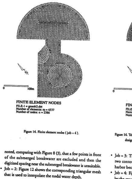
FINITE ELEMENT NODES

RLE-l=gmeshidat Number of elements: m o 4537 Number of nodes: n » 2386

FINITE ELEMENT GRIDS

FILE-l=gmesh2.dat

Number of elements: m=4537 Number of nodes: n » 2386

Figure 14. Finite element nodes (job = 4).

noted, comparingwith Figure 8 (3), that a fewpoints in front

of the submerged breakwater are excluded and then the

digitized spacing near the submerged breakwater is unsuitable.

Job = 2: Figure 12 shows the corresponding triangular mesh

that is used to interpolate the nodal water depth.

Figure 16. Triangular dement mesh for the linear finite element analysis,

designed for waves with the period of 10 sees. (job - 5).

Job = 3: The depth contours are shown in Figure 13. Only

two contour lines (10, 20m), in this case, are drawn in the

harbor because the sea bottom is flat in the other regions.

Job = 4: Figure 14 shows the finite element nodes indicated

(20)

CONTOURS: WATER DEPTH (Interpolated)

FILE-l = gmesh2.dat

Offshore water depth: hO = 20.00 in

Figure 17. Depth contours for the interpolated bathymetric data (job = 6 ).

CONTOURS: WAVE HEIGHT DISTRIBUTION FILE-l = gmesh2.dat

FILE-2 a waves2.dat Wave period: T = 10.00 sec Incident angle: THI = N45E

Job = 5: Figure 15 shows three kinds ofparticularly generated mesh in this example, defined in Chapter 2: GeneralRulesfir Mesh Generation. The triangular element mesh for the linear finite element analysis is shown in Figure 16. Note that the central mesh regions I-III in Figure 9, except for three particular mesh shown in Figure 15, are formed by nearly equilateral triangles. This mesh is designed for waves with the period of 10 seconds. The element mesh size is about 1/15-1/18 of the local wave length in the semicircular region ofthe harbor and

1/20 in the other regions.

Job = 6: The depth contours for interpolated bathymetric data

are shown in Figure 17, where there are two contour lines in the harbor. The contour line for 10m water depth is correct but that for 20m water depth is wrong because it should be a

straight line. The reason ofobtaining the zigzaz contour comes

from the fact that the corresponding region is not subdivided along the depth contours. This is an example of unsuitable subdivision of the bathymetric region of interest. Therefore, this indicates that in order to get correct depth contour lines,

the wave field of interest should be subdivided by using the

depth contour lines and the shorelines.

Job = 7: Figure 18 shows the comparison of the contours for

the wave height distribution ofthe linear wave analysis in terms of (1) the infinite element and (2) the coupling method. When the wave height relative to the incident wave height is greater

than or equals 1.0, the contours are drawn by the solid line

and when less than 1.0, by the broken line. The interval ofthe

contours is 0.2. The thick arrow shows the direction ofwave

incidence. Though there existsa little discrepancy chiefly nearby

the harbor mouth, these results are agree well with each other.

(1) Evaluated in terms ofthe infinit element.

CONTOURS: WAVE HEIGHT DISTRIBUTION FILE-l = groesh2.dat

FILE-2 *» wavesldat Wave period: T = 10.00 sec Incident angle: TH1=N45E

(2) Evaluated in terms of the coupling method.

(21)

28 TSUTSUI : CATWAVES, Prediction of Linear and Nonlinear Wave Motion in Unbounded Coastal Domains

/ / /// >' / / //■■'' .■ /

/

////////////

//

/ / / / / / / / / / / / / / / / •-'-•■ -~ 100m

CONTOURS: WATER DEPTH (Digitized)

FILE-1 =dcpth2.dat

(1) Combined with batymecric data (job = 3).

CONTOURS: WATER DEPTH (Interpolated)

RLE.legmesh2.da!

Offshore water depth: hO = 20.00 m

(2) Combined with generated element mesh data (job = 6). Figure 19. Wave rays on the two lands ofdepth contours.

The partial standing waves formed in front of the straight shoreline (y = 0) and the submerged breakwater are clearly seen. With the aide ofpartial wave reflection by the submerged breakwater, the wave field in the harbor seems to become calm compared with the normal condition ofwave incidence. • Jobs = 3, 6: As the further illustration of graphics, Figure 19

shows an example of combination of the wave ray trajectory due to refraction with the depth contours obtained from (1) bathymetric data and (2) the generated element mesh data. The angle ofwave incidence, in this case, is 45 degrees. Wave rays are refracted at the edge of the submerged breakwater and when reaches to the shoreline, stop propagation. Combination of the wave ray trajectory with bathymetric data, Figure 19 (I), is usual for checking incidence ofwaves. On the contrary,

combination with generated element mesh is sometime

valuable for investigation ofwave rays together with the wave height distribution.

■ Routine 9: Graphics II - Cross Sections Purpose

This routine generates data for the values ofwater depth and wave height at any specified point and their cross sections, which

are available for commercial-base software. Options

For digitized bathymetric data ("depth2.&&&"):

• job = 1: Evaluation of the water depth at any point.