境界要素法による単一液滴の物質移動解析 Computations of Mass Transfer from a Single Drop
by Boundary Element Method 秋元梢, 本間俊司, 古閑二郎, 松本史朗
Kozue AKIMOTO, Shunji HOMMA, Jiro KOGA and Shiro MATSUMOTO
Unsteady mass transfer from a two-dimensional drop is solved numerically with boundary element method. The domain is decomposed into two sub-domains for cylindrical drop and surrounding fluid, and boundary elements are arranged between the sub-domains. The system equation for boundary elements is derived by a direct method and by a finite difference approximation for time derivative. The solutions are independent of the number of elements on the interface of the drop and the external boundary of the domain.
The number of meshes inside the domain, on the other hand, affects the numerical solutions. It is necessary for good approximation to select appropriate resolution of the computational domain and the time step.
Keywords: boundary element method, drop, mass transfer
1.はじめに
単一液滴の物質移動は、液液抽出などの分離操作に おいて基礎となる重要な現象である。これまで、球状 で変形しない液滴を仮定した解析は多いが1)、変形を伴 う非定常運動のもとで物質移動を解析した研究例は少 ない。
変形を伴う液滴の非定常運動の解析においては、界 面運動の式を数値的に解く直接シミュレーションが行 われるようになってきた2)。物質移動に関する支配方程 式を流れの式と同時に解けば、原理的には非定常の濃 度分布も同時に得られる。しかしながら、物質移動に おける特性長さのスケールと流れのそれとは一般に大 きく異なり、液滴の非定常運動と物質移動を同時に精 度良く解析することは難しい。物質移動速度を精度よ
く求めるためには、非常に高い解像度を必要とする。
例えば、二酸化炭素が水に吸収される場合、濃度の計 算に必要な解像度は、流れの計算に必要な解像度の少 なくとも千倍高くする必要があると言われている3)。
我々は、界面運動および物質移動を、同時に精度良 く扱うことのできる数値解析手法を開発するため、液 滴 の 変 形 を 伴 う 流 れ の 解 析 に 、 有 限 差 分 /
Front-Tracking法
4)を、物質移動の解析に境界要素法をそ れぞれ用いたハイブリット型の計算コードの開発を目 指している。本研究では、開発の初期段階として二次元非定常拡 散方程式を境界要素法で離散化し、その近似解と液滴 周りの要素の分割数、外部境界の要素の分割数、およ び領域内部の解像度との関係を調査する。
2.定式化
2.1
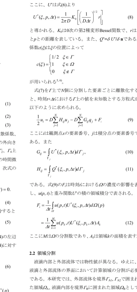
境界要素法による離散化Figure 1
に示すように、境界Γで囲まれた閉領域Ω内の任意の点
p(x, y)
において濃度分布u(p, t)
が二次元拡散 埼玉大学 工学部 応用化学科Department of Applied Chemistry, Faculty of
Engineering, Saitama University, 255 Shimo-Okubo,
Sakura-ku, Saitama, 338-8570, Japan
方程式
2
( , ) u D u p t
t
∂ = ∇
∂ p ∈ Ω , (1)
( ) ,
u p t = u p ∈ Γ Γ
1,
3, (2)
( ) ,
q p t = q p ∈ Γ Γ
2,
4(3)
によって記述される系を考える。ここにD
は拡散係数、q
は拡散流束でq =
∂u/
∂n
で定義される。n
はΓの外向き 法線ベクトルである。u
はΓ1、Γ3上で、q
はΓ2、Γ4上 でそれぞれ規定される既知関数である。式(1)
の時間微 分が、十分に小さい時間ステップ∆tについて、次式の ように差分近似できると仮定すると、2
1 1
( , ) ( , ) ( , ) 0.
u p t t u p t t u p t
D t D t
∆ ∆
∆ ∆
∇ + − + + =
(4)
式(4)に重み関数U
*(ξ, p, t)をかけて領域Ωで積分すると
*
( , , ) ( ) 0.
AU p t d p
Ω
ξ ∆ Ω =
∫ (5)
ここにξは観測点の位置を表す。また、
A
は式(4)
の左辺 である。部分積分を利用し、さらに、U
*が式(4)
に対す る基本解、2 *
1
*( , , ) ( , , ) ( , )
D U p t U p t p
ξ ∆ t ξ ∆ δ ξ
∇ − ∆ = − (6)
を満足する事を考慮すれば、式(5)は
( ) ( , ) ( , )
*( , , ) ( )
c u t t D u p t t Q p t d p
Γ
ξ ξ + ∆ = ∫ + ∆ ξ ∆ Γ ( , )
*( , , ) ( ) D q p t t U p t d p
Γ
∆ ξ ∆ Γ
− ∫ +
1
*( , ) ( , , ) ( ).
u p t U p t d p
t
Ωξ ∆ Ω
+ ∆ ∫ (7)
ここに、U*は式(6)より
1/ 2
*
0
1 1
( , , )
U p t 2 K r
D D t
ξ ∆
π ∆
= (8)
と導かれる。
K
0は0
次の第2
種変形Bessel
関数で、r
はξ とp
との距離を表している。また、Q
*=δ U
*/δ n
である。係数
c(ξ)
はξの位置によって1/ 2
( ) 1 0 c
ξ Γ
ξ ξ Ω
ξ Γ
∈
= ∈
∉
が用いられる5, 6)。
式
(7)
をΓ上でN
個に分割した要素ごとに離散化する と、時刻t+∆t
におけるΓ上の値を未知数とする方程式が 以下のように求められる。1 1
1
2
iN N
i ij j ij j
j j
u D H u D G q F
= =
= ∑ − ∑ + (9)
ここに
i
は観測点x
の要素番号、j
は積分点の要素番号で ある。また( )
*
, , ,
j
ij i j
G U ξ p t d Γ
Γ
= ∫ ∆ (10)
( )
*
, ,
j
ij i j
H Q ξ p t d Γ
Γ
= ∫ ∆ (11)
である。式
(9)
のF
iは時刻t
におけるΩの濃度の影響を表 し、u(p, t)
と重み関数U
*の積の領域積分で表される。1
*( , ) ( , , ) ( )
i i
F u p t U p t d p
t
Ωξ ∆ Ω
= ∆ ∫
* 1
1
M( , )
k( ,
i k, )
kk
u p t U p t A
t ξ ∆
∆
== ∑ (12)
ここにMはΩの分割数であり、
A
kは領域kの面積を表す。2.2
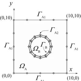
領域分割液滴内部と外部流体では物性値が異なる。ゆえに、
液滴と外部流体の界面において計算領域の分割が必要 である。本研究では、外部流体を境界ΓA1
, Γ
A2で囲まれ た領域ΩA、液滴内部を境界ΓBに囲まれた領域ΩBとして 全計算領域を分割した(Fig. 2)。2つの領域は境界ΓA2および
Γ
Bで接し、これらを内部境界と呼ぶ。部分領域ΩAおよびΩBにおいてそれぞれ境界要素方 程式が成り立つ。これをマトリックス形式で表すとΩA
に関しては、
Fig. 1 Computational domain.
1 1 1
1 2 1 2
2 2 2
.
A A A
A A A A
A A A
= −
U Q F
H H G G
U Q F (13)
一方、ΩBに関しては、
B
.
B
=
B B−
BH U G Q F (14)
マトリックスの要素は式
(9)
-(12)
より求めた。ΩAおよ びΩBの内部境界面ではu
が連続(適合条件)、q
が平衡(平衡条件)である。内部境界面の適合条件は次のよ うに表される。
2
.
A
=
B=
IU U U (15)
ここにUIは内部境界面における濃度を表す。また、平 衡条件はΩAおよびΩBにおける拡散係数をそれぞれ
D
Aおよび
D
Bとおくと以下の式で表される7)。2
.
A A B I
B
D
= − D =
Q Q Q (16)
ここに
Q
Iは内部境界面における拡散流束を表す。式
(15)
、(16)
を式(13)
、(14)
に結合条件として代入して 整理すると、1 1
1 2 2
1
1 2
0 0 0
0 0 0 0
0
A A
A A A
A
I A A
B B B
I B
A
D D
−
= −
U F
H H G
U G Q F
H G
Q F
(17)
となる。3.
結果と考察境 界 条 件 を
Γ
A1上 でu=0
、 初 期 条 件 をu(p, 0)=0
(
p ∈ Ω
A)、u(p, 0)=100
(p ∈ Ω
B)として解析を行った。時間刻み∆tは0.1とした。また、拡散係数はDA
=D
B=10
とした。Figure 3にp(5, y)におけるy方向の濃度分布の時間変
化を示す。図中の矢印の方向は時間が増加する方向で ある。時間とともに、濃度が0に収束している。外部境 界のuを0に固定しているのでこの収束値は物理的に正 しい。
Figure 4にt=2.0における濃度分布を示す。液滴中心か
ら外部流体へと物質が拡散している様子がわかる。Figure 5に液滴中心、すなわちΩ
B内の点(5, 5)におけ る濃度の時間変化をΓA2およびΓB(液滴周り)の要素分 割数ND毎に示す。図より液滴周りの要素分割数は濃度Fig.3 Concentration profiles at p(5, y).
Fig. 2 Domain decomposition and boundary elements.
Fig.4 Concentration distribution at t=2.0.
の時間変化に影響を与えないことがわかる。
Figure 6に点(5, 5)における濃度の時間変化をΓ
A1(外 部境界)の要素分割数N毎に示す。図よりNを変化させ ても結果に影響しないことがわかる。以上より、要素 の分割数は数値解に影響を与えないことがわかった。Figure 7
に領域の分割数M
を変化させた時の点(5, 5)
における濃度変化を示す。図より、濃度の時間変化は 計算領域の解像度よって変化することがわかる。M=10
×
10
の時、時刻t=0.1
で濃度が0
へ収束しているのは、内 点の解像度が不足しているためと考えられる。これはM=20
×20
へと解像度を上げることで解決した。一方、解像度が高い場合(M=30×
30
、M=40
×40
、M=50
×50)、
濃度のアンダーシュートがみられる。これは、解像度 を上げることによって、拡散流束の見積もりが大きく なったためと考えられる。
式
(8)
のBessel
関数は、引数が0
に近づくにつれ無限大 に発散する。領域の分割数を上げることによって、式(8)
のr
が小さくなり、U
*は非常に大きくなる。そのため、式
(17)
の右辺第二項が大きくなり拡散流束も大きくな る。これを解決するためには∆tを小さくし、式(8)
のBessel
関数の引数を大きくすればよいが、同時に式(12)
の
F
iが大きくなるため調整が必要である。精度良い解を得るためには、式
(8)
のBessel
関数の引 数r/(D∆t)
1/2を4
以上または0
に非常に近くする必要があ るとの報告がある7)。解像度M = 20×20においては、最小のr/(D∆t)1/2が0.5で、解像度が低いため、r/(D∆t)1/2 が4以上になる点も多い。一方、M = 50×50では引数 の最小値が0.2よりも小さく、かつ解像度が高いため、
引数が4に満たない点が多いと考えられる。
以上より境界要素法で非定常拡散問題を解く場合、
Bessel
関数の引数に注意し、適切な解像度と時間刻みを選定する必要があることが示唆された。
4.
結論単一液滴の界面運動および物質移動の同時高精度解 析を目指した研究の一環として、二次元非定常拡散問 題の境界要素法による解析を試みた。境界要素法によ る離散化においては、非定常項に差分近似を適用する
Fig.6 Time dependent concentrations at p(5,5) with the number of elements in Γ
A1. Fig.5 Time dependent concentrations at p(5, 5)
with the number of elements in Γ
A2and Γ
B.
Fig.7 Time dependent concentrations at p(5,5)
with the number of meshes in Ω
A.
方法で定式化した。試計算の結果、液滴周りの要素の 分割数および外部境界の要素の分割数は、数値解に影 響を与えなかった。一方、領域内部の解像度が数値解 に影響を与えることがわかり、基本解の形式が原因で あることを明らかにした。境界要素法を用いて非定常 物質移動現象を解析するためには、拡散係数に適した 解像度および時間刻みを選定する必要があり、さらな る検討が必要であることがわかった。
謝辞
本研究は、平成
15
年度埼玉大学教育研究推進費(学 長裁量経費)およびカシオ科学振興財団(平成16
年度 研究助成)から支援を得て行われた。参考文献