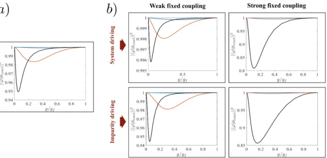
Composite Few‑Body System
Author Alan Kahan, Thomas Fogarty, Jing Li, Thomas Busch
journal or
publication title
Universe
volume 5
number 10
page range 207
year 2019‑10‑07
Publisher MDPI
Rights (C) 2019 The Author(s) Author's flag publisher
URL http://id.nii.ac.jp/1394/00001151/
doi: info:doi/10.3390/universe5100207
Creative Commons Attribution 4.0 International(https://creativecommons.org/licenses/by/4.0/)
Article
Driving Interactions Efficiently in a Composite Few-Body System
Alan Kahan
1,2, Thomás Fogarty
1,* , Jing Li
1and Thomas Busch
11
Quantum Systems Unit, Okinawa Institute of Science and Technology Graduate University,
Okinawa 904-0495, Japan; kahanalan@gmail.com (A.K.); jing.li@oist.jp (J.L.); thomas.busch@oist.jp (T.B.)
2
Instituto de Física Enrique Gaviola, CONICET and Universidad Nacional de Córdoba, Ciudad Universitaria, Córdoba X5016LAE, Argentina
* Correspondence: thomas.fogarty@oist.jp
Received: 30 August 2019; Accepted: 1 October 2019; Published: 7 October 2019
Abstract: We study how to efficiently control an interacting few-body system consisting of three harmonically trapped bosons. Specifically, we investigate the process of modulating the inter-particle interactions to drive an initially non-interacting state to a strongly interacting one, which is an eigenstate of a chosen Hamiltonian. We also show that for unbalanced subsystems, where one can individually control the different inter- and intra-species interactions, complex dynamics originate when the symmetry of the ground state is broken by phase separation. However, as driving the dynamics too quickly can result in unwanted excitations of the final state, we optimize the driven processes using shortcuts to adiabaticity, which are designed to reduce these excitations at the end of the interaction ramp, ensuring that the target eigenstate is reached.
Keywords: shortcuts to adiabaticity; cold atoms; few-body systems
1. Introduction
The ability to precisely control quantum systems is a prerequisite for developing technologies in the areas of quantum computation, simulation, and metrology. Even though the control over single-particle states is highly developed by today [1–3], the requirements stemming from short decoherence time-scales are often hard to fulfill. Even more so, fast operations can have detrimental effects on quantum states, as possible imperfections in the control pulses can be difficult to compensate.
To mitigate these problems, and to ensure high fidelity on short timescales, a number of techniques have been developed, such as optimal control algorithms [4–6] and shortcuts to adiabaticity (STAs) [7–11].
In this work we will focus on STAs, which are techniques designed to determine the driving parameters such that the system undergoes adiabatic evolution within a finite time, and which have been successfully employed in recent experiments with cold atoms [12–17]. While for single particles or within a mean-field approximation, the description of the exact evolution of the quantum state is tractable, extending such a treatment to interacting many-body systems poses complications due to their complexity. One solution is to use approximate variational techniques, and even though they are not exact, use these to design STA processes [18–20]. In fact, it has recently been shown that such an approach can be used to control correlations in small systems [21] and can serve as a good benchmark for the control of larger interacting systems.
In this work, we aim to move beyond mean-field and single-particle physics to control the dynamics of larger systems with short-range contact interactions. To achieve this, we take a first step by focusing on nontrivial few-body states, in particular, controlling the interactions in a bosonic two-component system confined to a harmonic trap. Such systems can exhibit complex dynamics arising from the interplay of intra- and inter-species interactions, leading, for example, to composite
Universe2019,5, 207; doi:10.3390/universe5100207 www.mdpi.com/journal/universe
fermionization or phase separation [22–25]. To discuss the basic effects, we will focus on a paradigmatic realization of a two-component system, namely, two interacting ultracold atoms of species A, which interacts with a single ultracold atom of species B in a one-dimensional setting. In such a system, the interactions can be described by point-like potentials, and in ultracold atom experiments, the interaction strength can be changed by employing Feshbach [26,27] or confinement-induced resonances [28]. In fact, individual tuning of the inter- and intra-species interactions allows one to explore driving the interactions of the A atoms in the presence of an impurity atom, driving the interaction between an impurity and the interacting A atoms, and also driving all interactions simultaneously. With this freedom, it is possible to explore driving the system through the phase separation transition, which can alter the ordering of the particles in the trap and, therefore, greatly affect the dynamics of the system. We will show that efficient STAs can be designed for the individual interactions based on a variational ansatz, and that these STAs can outperform a non-optimized interaction ramp for most timescales of the driven process.
In Section 2, we introduce the few-body model we consider, and in Section 3, we describe the variational method for designing STAs in this system. We begin in Section 4 with the analysis of driving interactions between three identical bosons, while in Sections 5 and 6, we investigate driving one of the interaction terms while the other is held fixed. These latter sections describe the effect phase separation has on the driven system and its dynamics. Finally, we conclude.
2. Model
We consider a one-dimensional system of three interacting bosons of mass m, confined in a harmonic trap of frequency ω, whose Hamiltonian is given by
H =
∑
3 j=1"
− ¯ h
2
2m ∇
2j+ 1 2 mω
2x
2j#
+ V
int( x
1, x
2, x
3) . (1)
At low temperatures, we can assume that the scattering between the particles is mostly two-body and of the s-wave form, allowing us to approximate the interaction part of the Hamiltonian with point-like pseudo-potentials as
V
int( x
1, x
2, x
3) ≈ g
A( t ) δ ( x
1− x
2) + g
AB( t ) [ δ ( x
1− x
3) + δ ( x
2− x
3)] . (2) Here, the interaction strength between two particles of species A is given by g
A, and the interaction strength between an A particle and the B particle is given by g
AB. Both couplings are related to the respective 3D scattering lengths, a
3D, via g =
4¯h2a3Dmd2⊥ 1 1−Cad3D
⊥
, with the constant C given by C ≈ 1.4603 [28]. Here, ω
⊥is the trap frequency in the transverse directions of a quasi-one-dimensional harmonic trap of width d
⊥= √
¯
h/mω
⊥, and one can see that control over the transverse trap frequency or the scattering length allows one to tune the interaction strengths. In the following, we will use harmonic oscillator units by rescaling all spatial coordinates with a
0≡ q
mωh¯, all interaction strengths in units of √
2a
0hω, all energies in units of ¯ ¯ hω, and time in units of ω
−1.
The Hamiltonian given in (1) can be separated by introducing Jacobi coordinates X = ( x
1− x
2) / √
2 , (3)
Y = ( x
1+ x
2) / √ 6 − √
2/3x
3, (4)
Z = ( x
1+ x
2+ x
3) / √
3 , (5)
where X and Y are two relative coordinates describing the positions of the three particles with respect to each other, while Z describes the system’s center-of-mass. The latter separates, and in these new coordinates, the Hamiltonian can be written as H = H
com( Z ) + H
rel( X, Y ) , with
H
com= −∇
2Z+ 1
2 Z
2, (6)
H
rel= − 1 2
∇
2X+ ∇
2Y+ 1 2
X
2+ Y
2+ g
Aδ ( X ) + g
AB"
δ − 1 2 X +
√ 3 2 Y
!
+ δ − 1 2 X −
√ 3 2 Y
!#
. (7) It is immediately clear that the center-of-mass part just describes a particle moving in a harmonic trap, for which the solutions are given by:
ψ
HOn( Z ) = π
−1/4( 2
nn! ) H
n( Z ) exp (− Z
2/2 ) , (8) where H
n( Z ) are the Hermite polynomials, and with energies E
n= ( n + 1/2 ) . The relative Hamiltonian can be interpreted as describing the effectively two-dimensional motion of a harmonically trapped particle in the presence of three narrow barriers arranged with a π/3 angle between them, as depicted in Figure 1a. Since the two A atoms are identical, the wave-function has to remain unchanged under a reflection across the X coordinate; however, there is no constraint when swapping particle B with one of the A particles. Exact solutions exist for limiting cases of the interactions [29,30], while in general, this system can be solved effectively using exact diagonalization techniques [24,31,32].
Indeed, for g
A6= g
AB, phase separation can be observed, whereby either the particles of species A are pushed to the edges of the trap, while particle B is confined in the trap center, or vice versa [23,32–35].
Therefore, the arrangement of the atoms in the trap is non-trivial and will be strongly affected by any change in their inter- or intra-species interactions. It makes this an ideal system in which to study all regimes of composite few-body dynamics and to develop useful quantum control techniques.
In the following, we will concentrate on increasing the interaction strength in initially non-interacting and uncorrelated systems on time scales t
f, which are approximately comparable to the trap period. As the center-of-mass contribution does not depend on the interaction, it will be unchanged during the interaction ramping process, and therefore, only the dynamics of the relative wave-function i¯ h
∂t∂ψ ( X, Y; t ) = H
rel( t ) ψ ( X, Y; t ) need to be considered.
For very slow ramps of the interaction (t
f≫ 1), the dynamics can be considered to be adiabatic, and the energy of the state after the process is equal to the energy of the eigenstate at the final value of the interaction strength, g
f, i.e., E
AD≡ E ( t
f) = E ( g
f) . For faster ramps (t
f∼ O ( 1 ) ), the process can be non-quasi-static, resulting in excess energy in the system due to the out-of-equilibrium dynamics, with non-adiabatic energy E
N A( t
f) ≥ E
AD. We can then define irreversible work from this non-adiabatic energy as
h W
irri = E
N A( t
f) − E
AD, (9) which for adiabatic processes will vanish, while being finite for non-quasi-static processes [21,36]. It is therefore a useful quantity to characterize the efficiency of the interaction ramp.
In the following, we will describe two kinds of interaction ramps. The first will be a generic, non-optimized reference ramp, which we will use as a benchmark and which we parameterize as
g
ref( t ) = g
f32
"
30 sin π 2
t t
f!
− 5 sin 3π 2
t t
f!
− 3 sin 5π 2
t t
f!#
. (10)
This function satisfies the boundary conditions g
ref( 0 ) = 0, g
ref( t
f) = g
f, and ˙ g
ref( 0 ) = g ˙
ref( t
f) =
¨
g
ref( 0 ) = g ¨
ref( t
f) = 0, ensuring that the interaction ramp begins and ends smoothly in an effort to
reduce untypical excitations. However, this assumption alone will not ensure that no irreversible
dynamics are created during the ramping processes, and the pulse can therefore serve as a reference to an optimized interaction ramp derived from the STA approach. This comparison will be our main tool to quantify the success of the designed STA, which we will develop in the next section.
3. Shortcut to Adiabaticity
To find an STA, we use the method of inverse engineering, which can design interaction ramps g
STA( t ) that fulfill the desired adiabatic evolution of the system φ ( X, Y; t ) for any ramp time t
f. The success of the STA then depends entirely on how well the solutions to the time-dependent Hamiltonian, φ ( X, Y; t ) , are known and whether they possess scale invariance [37]. As our interaction ramp is not scale invariant and since exact forms of the solution are not known, one has to use approximate techniques [19,38,39], and we therefore employ a variational approach with an ansatz that describes the evolution of the relative wave-function by an interpolation between the initial and the final state
φ ( X, Y; t ) = ϕ ( X, Y; t ) e
i(
b(t)X2+c(t)Y2) (11)
= N ( t ) h ( 1 − η ( t )) φ
i( X, Y ) + η ( t ) φ
f( X, Y ) i e
i(
b(t)X2+c(t)Y2) . (12) Here, N ( t ) is a time-dependent normalization constant, while b ( t ) and c ( t ) are chirps that allow the wave-function to change its width. To ensure that the wave-function changes smoothly from the initial state φ
i( X, Y ) ≡ φ ( X, Y; g
i) to the target state φ
f( X, Y ) ≡ φ ( X, Y; g
f) , we choose η ( t ) as a 6
thorder polynomial satisfying the boundary conditions η ( 0 ) = 0, η ( t
f) = 1 and ˙ η ( 0 ) = η ¨ ( 0 ) = η ˙ ( t
f) =
¨
η ( t
f) = 0.
Figure 1. (a) Interaction potentials stemming from g
A(dashed line) and g
AB(solid lines) in the Jacobi coordinate plane. (b) Examples of different interaction ramps when keeping g
A( t ) = g
AB( t ) , with the reference ramp (blue dotted line) and the shortcut to adiabaticity (STA) ramp at t
f= 1.5 (black solid line) and t
f= 10 (red solid line).
The next step in the process is to minimize the action of the effective Lagrangian [18]
L = Z
∞−∞
dX Z
∞−∞
dY
"
i 2
∂φ
∂t φ
∗− ∂φ
∗
∂t φ
− 1 2
∂φ
∂X
2
− 1 2
∂φ
∂Y
2
− V ( X, Y; t ) | φ |
2#
, (13)
where V =
12X
2+ Y
2+ g
A( t ) δ ( X ) + g
AB( t ) h δ
−
12X +
√3 2
Y
+ δ
−
12X −
√3 2
Y i
contains the
trapping and the interaction potentials. This effective Lagrangian is minimized with respect to the
variational parameters η ( t ) , b ( t ) , and c ( t ) , and the resulting Euler–Lagrange equations give the
evolution equations that will determine b ( t ) and c ( t ) and establish the time dependence of the two interaction strengths, g
A( t ) and g
AB( t ) , given by
g
A( t ) I
A+ g
AB( t ) I
AB= − ∂ξ
2∂η
b ˙ + 2b
2+ 1 2
+ ∂ν
2
∂η
˙
c + 2c
2+ 1 2
+ 1
2
∂
∂η ( β + γ )
. (14) Here, ξ
2= R
∞∞
dX R
∞∞
dY X
2| ϕ |
2and ν
2= R
∞∞
dX R
∞∞
dY Y
2| ϕ |
2are the widths of the state in the X and Y directions, respectively, and their dynamics is determined by
ξ ˙ = 2bξ, (15)
˙
ν = 2cν. (16)
Similarly, the kinetic energies in these directions are β = R
∞∞
dX R
∞∞
dY
∂ϕ
∂X
2
and γ =
R
∞∞
dX R
∞∞
dY
∂ϕ
∂Y
2
, and the interaction energies are I
A= R
∞∞
dX R
∞∞
dYϕδ ( X ) and I
AB= R
∞∞
dX R
∞∞
dYϕ h δ
−
X2+
√ 3 2
Y
+ δ
−
X2−
√ 3 2
Y i
. Using known solutions to φ
iand φ
fallows us to calculate these terms exactly (for example, in the limit of infinite repulsive interactions, accurate approximations are known [29,30]); otherwise, these integrals can be calculated numerically. Typical examples of these STA interaction ramps for a system of three identical particles are shown in Figure 1b for two timescales t
f= { 1.5, 10 } . When t
fis large, the STA is designed to quickly ramp the interaction at the end of the process, in contrast to the reference, which begins to slowly increase the interaction already at the beginning of the ramp. This difference is due to the optimization of the STA through the Lagrangian, which is designed taking into account the energy dependence on the interaction and is similar to that seen in smaller systems [21]. For small t
f, the STA possesses large modulations as driving the system faster requires large changes in the energy to follow the adiabatic path.
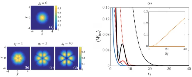
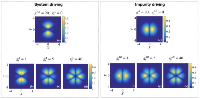
4. Three Identical Particles
Assuming that the initial state is the ground state of the noninteracting system, g
i= g
iA= g
ABi= 0 (see Figure 2a), we investigate in the following the ramping of strong interactions between three identical particles, i.e., g ( t ) = g
A( t ) = g
AB( t ) . In this case, the relative part of the wave-function will always possess C
6νsymmetry [31,40,41] (see Figure 2b–d), with the interactions leading to cusps in the density at 60
◦angles to each other, and with the cusp asymptotically reaching zero density in the Tonks–Girardeau limit of strong repulsive interactions (g
f& 40) [42–44].
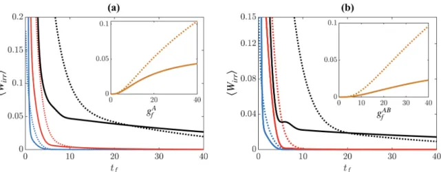
To quantify the success of the interaction ramps, we compare the irreversible work h W
irri after the respective interaction ramps (see Figure 2e). For longer ramp times, t
f> 25, the system is driven slowly enough that it can be considered as evolving adiabatically, which results in a vanishing h W
irri and therefore, a high-fidelity process for any reasonable non-optimized reference ramp. However, for short ramp times, t
f. 10, ramping to stronger interactions creates more irreversible dynamics as the system is driven further from its equilibrium, resulting in large h W
irri and therefore, low-fidelity final states. It is on these timescales that we see the advantages of using the STA as it outperforms the non-optimized reference ramp, possessing lower amounts of h W
irri for the different final interactions.
The modulations visible in h W
irri for the STA are due to excitations of the system to high energy states
that possess the same symmetry as the ground state. While the contribution of these excitations is
small for long ramp times, when driving the system quickly the STA is unsuccessful in damping them
due to its approximate form through the ansatz in Equation (11). Indeed, divergence of h W
irri occurs
for timescales t
f. 1, when the STA ramp becomes negative at certain time intervals and destabilizes
the system. This sets a limitation on the operation of our STA to times t
f> 1.
Figure 2. (a) Initial state in the relative { X, Y } coordinate plane. Target states at (b) g
f= 1, (c) g
f= 5, and (d) g
f= 40. (e) h W
irri for three indistinguishable particles as a function of the ramp time t
ffor the STA (solid lines) and reference ramp (dotted lines). The final interactions are g
f= 1 (blue lines), g
f= 5 (red lines), and g
f= 40 (black lines). Inset shows h W
irri versus final interaction strength g
fat t
f= 10.
While for ramps to weak interactions the STA and the reference give comparable results, the difference between them increases when driving to larger interactions (see inset of Figure 2e).
When using the STA, the final state is essentially reached with t
f= 10 for any final interaction;
however, applying the reference ramp drives the system further from the target eigenstate with growing interactions. This is not surprising as driving quickly to an infinitely repulsive state results in a diverging energy expectation value [45,46]; however, in this case the STA allows us to drive the system significantly faster than the reference as the excitations are successfully suppressed.
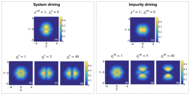
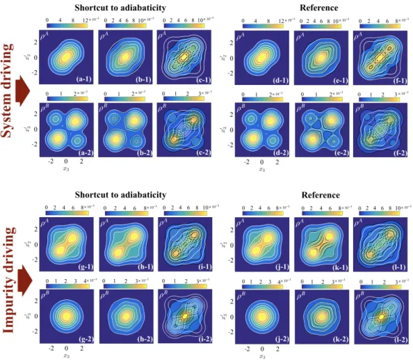
Finally, we compare the structure of the three-body state through comparisons of the one-body density matrix (OBDM), whereby we examine the reduced state after tracing out two particles from the system
ρ
A( x
1, x
01) = Z
+∞−∞
Ψ ( x
1, x
2, x
3) Ψ
∗( x
01, x
2, x
3) dx
2dx
3, (17) ρ
B( x
3, x
03) =
Z
+∞−∞