47
Exploration of Economic Growth Analysis of Singapore : Construction of Historical GDP Estimates (1900-39 and 1950-60) and Empirical Investigations —Brief Summary—
Ichiro SUGIMOTO
1. Outlines of Contents
This paper is organized as follows. Section 2 identifies the significance of the construc- tion of historical GDP estimates and its empirical investigation as a new branch of economic analysis of Singapore. Section 3 briefly sketches out the methodologies employed for the construction of each component of GDP in both current and constant prices. Section 4 describes major findings on the overall patterns of Singapore's GDP. Findings on two types of empirical investigations relating to long-term economic growth of Singapore are provided in Section 5.- Lastly, limitations of this study and the area of future research area are outlined in Section 6.
2.: Significance of This Study •
In OECD countries, studies on long-term economic growth were regarded as one of the dynamic branches of economics. The development of this branch of study had been closely associated with the construction of economic related data which conform to the definition of
"The System of National Accounts (SNA)". Historical statistical data was scrutinized and recompiled in the form of national accounts and its validity was tested.
Unlike developed nations, very few studies of similar nature were made in the developing countries. This existing research gap between developed and developing countries could mainly be attributed to the lack of statistical information in the case .of the latter. More importantly, the absence of local experts who could initiate these types of exercises was another major obstacle as 'commented by Simon Kuznets (Oshima, 1997).
To quantify the economic performance, some studies alternatively used "size of trade"
as a proxy to measure economic development while acknowledging that these variable was not a reliable proxy to indicate economic growth. This implies that deficiencies of the relevant economic indicators do not permit the conduct of modern quantitative economic analysis..
In Singapore, official GDP figure was released since 1960. For the period 1960-2000, real
48 S~1 • IRE AlAatVol. XLI, No. 1-2-3-4
GDP (1990 prices) rose at an average annual rate of. 7.7 percent. With population growth at 2.2 percent, real per capita GDP increased by 5.5 percent on average each year. In fact , real
per capita GDP has increased 9.7 times within 40 ' years. Out of 107 countries, Singapore registered the highest growth performance during the period 1960-2000 (Ghesquiere 2007 : 14)..
Reflecting this notable economic growth, many empirical studies have been conducted by
local and foreign researchers.
Unlike the period after 1960, the literature on economic history prior to 1960 on Singapore was somewhat different. In fact, the studies on the economic history of Singapore approached
from various aspects ranging from trade, commercial activity, money, government finance' and financial development to economic conditions during the world depression. Apart from
this, studies on demographic changes, labour conditions, infrastructure development such as
water supply and port facilities were also conducted. Additionally, the economic importance of Singapore as an entrepot and a regional trading centre was often highlighted . The first
major research work conducted by Huff, W.G (1994) traces the long-term economic develop- ment of Singapore as an economic entity during the twentieth century . "The history of Singapore is . written mainly in statistics" is the opening sentence in Huff's book . Huff had
immersed himself in the collection and integration of the statistical material from a host of
primary, secondary and even obscure data sources. His studies mentioned above have, in fact,
immensely contributed in towards a deeper understanding of the economic history of Sin- _ gapore. However, his scope of research was basically determined by the availability of the
• • relevant statistical information compiled by the British colonial authority .
In a literature review on the economic history of Malaya (inclusive of Singapore) made by Wong Lin Ken (1979) under the title of "Twentieth-Century Malayan Economic History :
A Select Bibliographic Survey", he stated that "research in this region is still on the frontier
area of* the social sciences. Analytical methodology grounded in economic theory was lack-
ing". Some two decades later, Drabble, John H (2000), in his book on Economic History of Malaysia which covered the period 1800-1990 elaborated the progress of economic history of Malaysia by stating that `from the standpoint of the economic historian the situation is still
to a large extent as Wong described". The above statements made by economic historians
made abundantly. clear that research in this field of economic history saw little progress in this part of region.
Based on this recognition, the collection and construction of macroeconomic time-series
data of Singapore such as GDP, which is an integral part of this study represents a fundamen-
tal but crucial step towards filling this void, notwithstanding the painstaking and tedious task
of compiling the required raw data from various official publications and records .
March 2012 Ichiro Sugimoto • 49
• I n terms of empirical investigation of economic growth of Singapore, this study .will reveal the economic performance of Singapore in quantitative terms. Unlike OECD countries, the foundation of Singapore economy was established during the British colonial period. It is significant to see whether there are any differences and similarities in economic growth between British the colonial period and that of the period of self-government.
One of the salient features of Singapore's economy is its high degree of openness to international trade. Basically, this nature of Singapore's heavy dependence on the interna- tional economic environment remains essentially unchanged until today. Given this scenario,
Singapore has been extraordinarily vulnerable to external shocks, whether it be a slowdown in export growth, a sharp exodus of short-term capital, a change in world interest rates, or an increase in imported inflation.
Another characteristic found in Singapore's economy was with regards to the govern- ment's fiscal behavior. This study was driven by the hypothesis that government finance behavior in relation to economic growth in Singapore might have experienced a significant shift due to the administrative changes brought about in the process of transition from British colonial rule to self-government. These kinds of research questions can only be empirically investigated when . long-term time-series data is available.
3. Construction of Historical GDP Estimates in the Twentieth Century
3.1 Methodology Employed for Estimation of Each Component of GDP for the period 1900-39 and 1950-60.
As compared with modern estimates of GDP, the construction of historical GDP esti-
mates has more serious constrains on the grounds that every step in the estimating procedure
would depend on the availability of statistical . information. Gathering and preparing of
statistical material into time-series database represents a basic but important step in
constructing GDP estimates. Ideally, estimates using the three different approaches, namely
production, income and expenditure approaches would be most desirable since reasonable-
ness of the results of these estimates can be evaluated one against the other. However, this
is again constrained by the availability of data. Based on the constraints of data availability
during the period under study (See Appendix Figure 1), it was decided to apply the expendi-
ture approach rather than production and income approaches to obtain GDP estimates of
Singapore. Various creative methodologies were applied but always consciously conforming,
as closely as possible, to the definitions as outlined in "The System of National Accounts
(SNA) 1968". The following sub-sections briefly provide the estimating procedures for each
component of GDP, namely Private Final Consumption Expenditure by resident households
50 Si1 fat g A got . AVol. XLI, No. 1.2.3.4 (PFCE), Government Final Consumption Expenditure (GFCE), Gross Capital Formation
(GCF) and Net Exports of Goods and Services.
3.1.1 Private Final Consumption Expenditure by Resident Household (PFCE)
Presently, household budget surveys and commodity flow tables are widely utilized for the computation of PFCE. However, these approaches 'could not be employed due to the
dearth of such data for the early period. Consequently, alternative techniques had to be
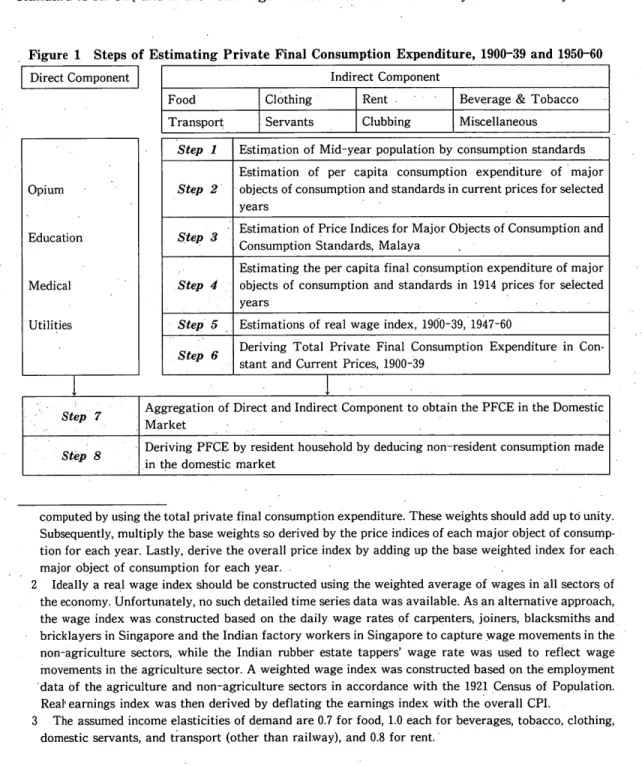
utilized in arriving at these estimates. As presented in Figure 1, two distinctive approaches
were employed viz the direct and indirect approach. In the direct approach, data on consump-
tion expenditure pertaining to opium, education, medical fees and utilities (gas, water supply
and electricity) was gathered independently from various official. sources. The indirect
approach involved the estimate of PFCE on food, beverages and tobacco, clothing, rent,
domestic servants and transport: Summing up the expenditures .derived from these two
approaches provides us the PFCE in current and constant prices.
The indirect approach estimates involved a number of steps. Firstly, six consumption
standards were classified based on the recognition that there are significant differences in consumption levels and expenditure patterns among the ethnic groups. Subsequently, the
current per capita consumption expenditure of each major object of consumption was
identified for each standard. These figures were then deflated by the consumer price indices
of each major object of consumption' to obtain the expenditure in constant prices. Real per
1 Consumer price index (CPI) forms a basis for measuring the rate of inflation and a useful tool for deflating PFCE, wage rates, etc. It provides a measure of the average rate of change in prices of.a fixed
basket of consumer goods and services which represents the household expenditure pattern. For this
purpose, CPI by major object of consumption was required to obtain the respective real per capita
consumption expenditure. Additionally, the overall CPI was utilized to compute real wage indices. The following actions were taken to compute the CPI.
Firstly, estimate the private final consumption expenditure of each major object of consumption for each consumption standard for the base year (1914=100). Secondly, compute the base weights of private
final consumption using the total private final consumption expenditure of each major object of consump-
tion by each consumption standard. The weights of private final consumption of each consumption . standard within a particular major object of consumption should add up to unity. Subsequently,. multiply
the base weights of private final consumption of each consumption standard within a particular major
object of consumption by the relevant price indices of each year. Based on the above procedures, derive
the overall price index of each major object of consumption by adding up the weighted index of each
standard. This would give you the overall price index for each major object of consumption for each year.
There are essentially two (2) series of price indices. The first series covering the period 1900-39 had 1914
as its base year (1914 =100) while the second series encompassing the period 1939, 1947-60 had 1949 as the
base year. With 1939 being common to both series of price indices, it was then possible to reconstruct one
continuous series for the period 1900-39 and 1950-60 with 1914 as the base year (1914=100) by using the
overlapping 1939 price indices expressed as a conversion factor and applying it to the period 1950-60. The
weights of PFCE in the base year of each major object of consumption (irrespective of standard) were
March 2012 Ichiro Sugimoto 51 capita consumption expenditure of each major object of consumption of each standard was then adjusted based on the changes in real income2 over time taking into account the income elasticities of demand by each major object of consumption3. For example, annual figures on PFCE for food for the European standard in both constant and current prices were computed as follows. If in the base year (t), the real per capita expenditure on food for European standard is RPCFt and if the real wage indices' increases from 1 in year t to 1.2 in year t+
Figure 1 Steps of Estimating Private Final Consumption Expenditure, 1900-39 and 1950-60
Direct Component Indirect Component
Food Clothing Rent Beverage & Tobacco
Transport Servants Clubbing Miscellaneous
Opium
Education
Medical
Utilities
Step 1 Estimation of Mid-year population by consumption standards
Step 2
Estimation of per capita consumption expenditure of major objects of consumption and standards in current prices for selected years
Step 3 Estimation of Price Indices for Major Objects of Consumption and Consumption Standards, Malaya
Step 4
Estimating the per capita final consumption expenditure of major objects of consumption and standards in 1914 prices for selected years
Step 5 Estimations of real wage index, 1900-39, 1947-60
Step 6 Deriving Total Private Final Consumption Expenditure in Con- stant and Current Prices, 1900-39
Step 7 Aggregation of Direct and Indirect Component to obtain the PFCE in the Domestic Market
Step: 8 Deriving PFCE by resident household by deducing non-resident consumption made in the domestic market
computed by using the total private final consumption expenditure. These weights should add up to unity.
Subsequently, multiply the base weights so derived by the price indices of each major object of consump- tion for each year. Lastly, derive the overall price index by adding up the base weighted index for each.
major object of consumption for each year. .
2 Ideally a real wage index should be constructed using the weighted average of wages in all sectors of the economy. Unfortunately, no such detailed time series data was available. As an alternative approach, the wage index was constructed based on the daily wage rates of carpenters, joiners, blacksmiths and bricklayers in Singapore and the Indian factory workers in Singapore to capture wage movements in the non-agriculture sectors, while the Indian rubber estate tappers' wage rate was used to reflect wage movements in the agriculture sector. A weighted wage index was constructed based on the employment data of the agriculture and non-agriculture sectors in accordance with the 1921 Census of Population.
Real' earnings index was then derived by deflating the earnings index with the overall CPI.
3 The assumed income elasticities of demand are 0.7 for food, 1.0 each for beverages, tobacco, clothing,
domestic servants, and transport (other than railway), and 0.8 for rent.
52 • 9I1 ti1 41 A r • Vol. XLI, No. 1.2.3.4 1, real per capita expenditure onfood in year t+ 1 (RPCFt+t) was calculated .as follows
RPCFt+i = RPCFt + ((RPCFt x 1.2/1.0)X 0.7)
If the real earnings index increases .to 1.5 in year t+2, per capita food expenditure in year t+2 was calculated as follows :
RPCFt+2=RPCFt+1+((RPCFt+i x (1.5-1.2)/1.2)) X 0.7))
Real per capita . expenditure of the European standard on food for the period 1900-39 was then multiplied by the population of each year of the European Standard to obtain the real PFCE of the European Standard on food for each reference year. The derived figures were then inflated by the food indices to arrive at the PFCE in current prices. Similar procedures were applied for each major object of consumption for the six consumption standards.
PFCE in the domestic market was then derived by aggregating the figures of the direct components and' indirect components. In . order to obtain PFCE by resident households, adjustments were made.
3.1.2 Government Final Consumption Expenditure
.Government final consumption expenditure (GFCE) was derived by deducting . from the government output (goods and services), the sales of other goods and services produced by the producers of government services. Output of producers of government services was computed by summing up the compensation of employees (personal emoluments), the intermediate consumption of goods and services and the depreciation allowances of all producers of government services. These estimates include the expenditure incurred by Colony of Sin- gapore, Municipality/City Council of Singapore and Rural Boards5. Detail expenditures recorded in conventional government accounts varied among administrative bodies and also within each administrative body over time.
To meet the definitions of SNA68, the following steps were taken to identify the government final consumption' expenditure. In general, the government expenditure accounts presented expenditure incurred by each department. Within the department, two major classifications were made, viz, personal emoluments (compensation of employees) and 'other charges (annual recurrent and special expenditure). Under this broad classification, details were provided. Unfortunately, no systematic presentation of the expenditure incurred was available. In view of this, it was necessary to set up a coding system that would identify for
4 Data on household income was not available. The movementsof the nominal weighted wage indices of the agriculture and non-agriculture sectors were then used as surrogates for household income changes.
The real wage index for the period 1900-39 was then computed by dividing the linked series from 1900 -39 by the overall Consumer Price Indices with base year 1914 =100 .
5 Military expenditure on capital formation items have been treated as intermediate consumption of
goods and services and form 'part and parcel of output. •
March 2012 Ichiro Sugimoto 53 our purpose, compensation of employees, intermediate consumption, capital formation, transfers and others. These standard procedures however, were not fully applicable for all
"
government accounts due to the deficiencies of data. Therefore, the following approach was applied based on the availability of data.
Firstly, information on revenue received by class of account was utilized to identify the sales of other goods and services by producers of government services. For the compilation of the government final consumption expenditure, the expenditure incurred by. the following departments were excluded : (i) Drainage and Irrigation Department, (ii) Electric Supply Department (iii) Gas Supply Department, (iv) Government Monopolies Department, (v) Post and Telegraph Department, (vi) Printing Department, (vii) Public Works Department, (viii) Railway Department and (ix) Water Supply Department.
'S econdly, from the producers'of government services, independent transfer items record- ed as a head of department such as pensions, purchase of land, payment of loans are also excluded. Having done these deductions, the output of producers of government services which constitute compensation of employees and intermediate consumption expenditure were
identified. .
Consumption of fixed capital, however, is very difficult to trace due to the dearth of data.
Therefore, based on the available post independence period information, it was assumed that 1% of gross output of producers of government services would be classified as depreciation
•
allowance.
Thirdly, government sales were deducted from gross output of producers of government services. Sales of other goods and services produced by the producers of government services
•
refer to the school fees, hospital fees,:etc.
3.1.3 Gross Capital Formation
The estimates of Gross Capital Formation (GCF) include investments made on construc- tion, machinery and equipment and cultivated assets. Inventories include stocks of goods. held by producers to meet temporary or unexpected fluctuations in production or sales, and work
in progress other than construction.. .
In the case of construction output capitalized, total construction output was firstly derived by using input-output coefficients of cement to total construction output based on the first construction survey in 1972. Total construction expenditure that went into fixed capital
formation was then derived by deducting from total output of construction, the expenditures incurred on repairs and maintenance.•
In the case of investment on machinery "and equipment (M&E), it was assumed that the
M&E produced locally during the period was negligible for the period under study. This
54 1Vol. XLI, No. 1.2.3.4 . means that total net imports valued at market prices was equivalent to total investments in M&E. Net imports of M&E at c.i.f. values were obtained from official trade statistics. No commodity taxes were levied against M&E which meant that the c.i.f. (basic) and producers' values were identical. Trade and transport margins were added to producers' value to arrive at market prices. The final step was to determine what proportion of net imports was to be capitalized. Some of these imports would have been used as inputs into construction activity and some as part of private final consumption expenditure.
In preparing the estimates on the. investment for cultivated assets, only rubber and coconut were selected since other perennial crops were found to be negligible. All expenses sunk into perennial crops prior to their reaching the bearing age were treated as part and parcel of capital expenditure. Three types of information were utilized for the above . computation, namely, .newly planted acreage for each year, number of years it takes for the crop to reach bearing age and annual cost per acre of bringing the crop into production. The yearly estimates of expenditure on cultivated assets at different years of maturity were derived by multiplying the total immature acreage with the . corresponding base year esti- mates of cost of investment per acre at different stages of maturity. These yearly estimates were then aggregated to arrive at the yearly estimates of real capital expenditure. Total real investment in cultivated assets was then inflated by the nominal rubber tapper's earnings indices (See . Figure 2). For both rubber and coconut, a distinction was made between smallholding , and estate cultivation..
Inventory as defined in SNA68, consists largely of raw materials and supply, finished or partly finished products awaiting sale and unpaid work in progress on assets which take a long time to produce. The colonial government records, however, did not provide sufficient Figure 2 Singapore : Format for Calculating Investment on Coconut Planting at Current
Prices, 1910-16
1910 1911 1912 1913 1914 1915 1916
Newly Planted Acreage for 1910 Cost per acre (1911 prices) Value
[1]
[2]
[A] = [1] x [2]
10 50
10 20
10 20
10 20
10 20
10 20
500 200 200 200 200 .,:200
Newly Planted Acreage for 1911 Cost per acre (1911 prices) Value
[3]
[4]
[B] = [3] x [4]
1910 1911
30 50
1912 30 20
1913 30 20
1914 30 20
1915 1916 30 30 20 20
1,500 600 600 600 600 600
Investment (1911 prices)
Rubber Tappers Indices (1911 prices) Investment (Current Prices)
[C]=[A]+[B]
[D]
[E] = [C] x [D]/100
1910 1911 1912 1913 1914 1915 1916
500 1,700 800 800 800 800 600
90 100 110 120 130 140 150
450 1,700 880 960 1,040 1,120 900 Rubber Tappers Indices (1914 prices)
Investment (1914 Prices)
[F]
[G] = [E]/[F]'100
69 77 85 92 100 108 115
652 2,208 1,035 1,043 1,040 1,037 783
March 2012 Ichiro Sugimoto55
information to construct reliable estimates. Under these serious constraints of data availabil- ity, the official figures available after 1960 were utilized. It was observed that there was a positive correlation between GDP growth and value of changes in stock. Based on the prevailing economic conditions as reflected in the level of GDP growth rate, the percentage contribution of changes in stock to GDP were assigned values ranging from —3.0% to 3.0%.
3.1.4 Exports and Imports of Goods and Services
Export and import statistics cover transactions of goods and services between the residents of one country and non-residents of another: Data on merchandize imports and exports of Singapore were available for the period 1900-27. For the periods 1928-39, 1950-60, W.G. Huff's estimates (1994) were applied. Estimates for exports and imports of services
were captured in this estimate by using port and other related statistics.
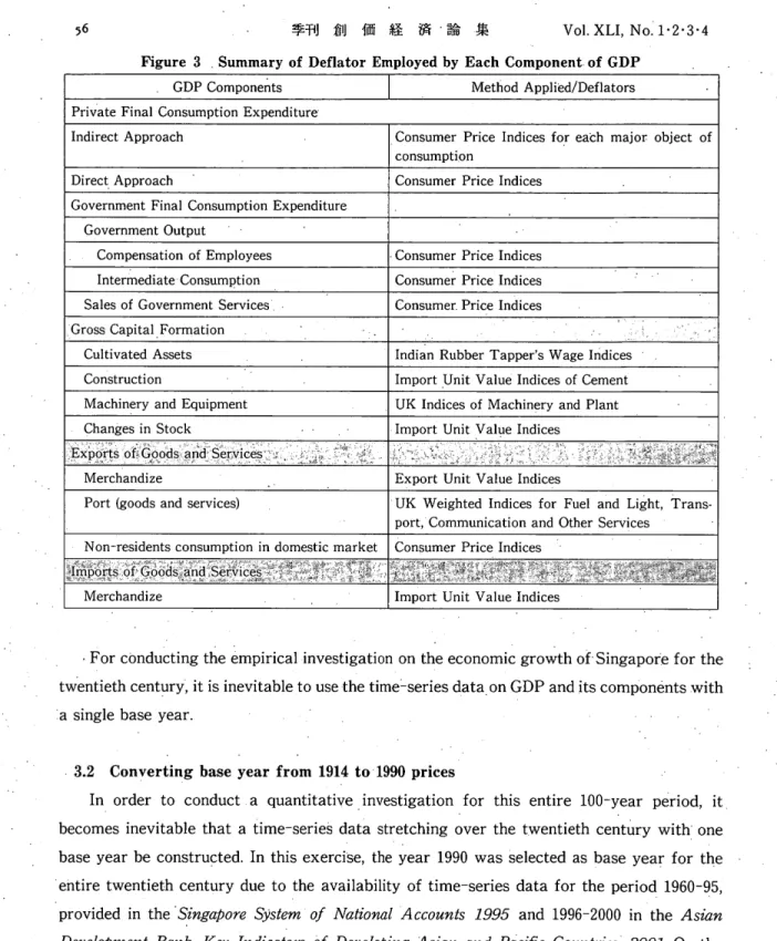
3.1.5 Deflators
Real GDP figures were arrived at by deflating each component of aggregate demand in current prices by various deflators into constant 1914 prices for the periods 1900-39 and 1950 -60 . Figure 3 portrays the various deflators used in the deflation process. For example, CPI and Import and Export Unit Value Indices were computed using the Laspeyres Price Indices'.
Unit values of commodities were derived from the quotients of values and quantities. As it was not feasible to derive an outright continuous unit value indices series due to changing composition of exports, the sample period was broken down into several but overlapping intervals with different base years. The criteria for the selection of intervals and their base years include relative stability of the shares of commodities and a relatively tranquil year. In this exercise, the base year of each interval is identified based on the proximity of. the price of the commodity that commands the largest weight to its average price level during the corresponding interval.
This method preserves the same growth rates of the .estimates associated with 1914 prices. For the new series in 1990 prices, the growth rates of each component of GDP, namely PFCE, GFCE, GCF, EXGS and IMGS for the years 1900-39 and 1950-60 correspond to the
1914 constant price series. However, the growth rates of GDP components in 1990 prices are different from that of GDP series in 1914 prices. Similarly, as would be expected, the percentage share of each component of GDP in 1990 prices was different from 1914 prices.
EPnQo — Po*PoQo 6 L aspeyres Price Indices computed using the following formula ; EPoQo EPoQo
where Pn = Price in current period .
Qo=Quantity in base period.
Currently, Department of Statistics, Singapore use Laspeyres Price Indices for CPI and Import and
Export Unit Value Indices.
56
•
211 (iig M •Vol. XLI, No. 1.2.3.4
Figure 3 . Summary of Deflator Employed by Each Component. of GDP
GDP Components Method Applied/Deflators
Private Final Consumption Expenditure
Indirect Approach Consumer Price Indices for each major object of consumption
Direct Approach Consumer Price Indices
Government Final Consumption Expenditure Government Output
Compensation of Employees Consumer Price Indices
Intermediate Consumption Consumer Price Indices
Sales of Government Services Consumer. Price Indices Gross Capital Formation
Cultivated Assets Indian Rubber Tapper's Wage Indices
Construction Import Unit Value Indices of Cement
Machinery and Equipment UK Indices of Machinery and Plant
Changes in Stock• Import Unit Value Indices
Exports of Goods and Services
• '-'- s • •Merchandize Export Unit Value Indices
Port (goods and services) • UK W eighted Indices for Fuel and Light, Trans- port, Communication and Other Services
Non-residents consumption in domestic market Consumer Price Indices irnports 01 uooas ,ana services
Merchandize Import Unit Value Indices
For conducting the empirical investigation on the economic growth of-Singapore for the twentieth century, it is inevitable to use the time-series data on GDP and its components with a single base year.
3.2 Converting base year from 1914 to 1990 prices
In order to conduct a quantitative investigation for this entire 100-year period, it
becomes inevitable that a time-series data stretching over the twentieth century with one
base year be constructed. In this exercise, the year 1990 was selected as base year for the
entire twentieth century due to the availability of time-series data for the period 1960-95,
provided in the 'Singapore System of National Accounts 1995 and 1996-2000 in the Asian
Development Bank, Key Indicators of Developing Asian and Pacific .Countries, 2001. On the
other hand, 1914 was selected as a base year for the periods 1900-39 and 1950-60. For
purposes of conducting rebasing from 1914. to 1990 prices for the period, 1900-39 and 1950-60,
the following formula was applied for re-scaling.
March 2012 Ichiro Sugimoto 57
zE so=zE14x~Eso
14Where =Ey is the estimate of year x in base year y prices.
PFCE and GFCE were deflated by CPI. On the other hand, other components of GDP were deflated differently. In the case of GCF, investment in cultivated assets, construction, transport, machinery and equipment and change in stock were deflated by a different deflator separately. Similar to this, merchandize trade and service trade were deflated by their respective deflators. Nevertheless, official database for the years 1960-2000 merely provides implicit deflators for each component of GDP. Under these constraints of availability of deflator, it was decided to apply the implicit deflators for GCF, EXGS and IMGS.
4. Overall Patterns. of Singapore GDP for the Twentieth Century
This first cut estimate of long-term historical GDP series helped in the overview of the economic performance of Singapore (See Table 1 and 2). In constant terms (1990 prices) , the annual average growth rates of GDP for the periods 1900-1939 and 1950-2000'were 4.4% and 7.2% while growth rates of real per-capita GDP for similar periods were 1.4% and 4.6%
respectively. Both results reinforce the historical fact that the overall growth rate of GDP during the post-World War II period was significantly higher than that of the pre-World War II period. A similar phenomenon is observed for each of the components of GDP. In the pre -independence period (1900-39 , 1950-64) the share of each component of GDP was relatively stable over time though there were occasional fluctuations. In the twentieth century, the most notable negative growth was recorded during the Great Depression period (1930-1932).
In contrast to this period, long-term structural changes were observed after the attain- ment of independence in 1965. In particular, private final consumption expenditure by resident households (PFCE) showed drastic falls from about 74 per cent. of GDP in the 1960s to around 40 per cent at the end of the 20th century. A large fall of PFCE can be explained by the remarkable increase in Gross Domestic Savings (GDS) over this long period (Peebles and Wilson, 2002 ; 78). This increase of the saving rate can be attributed to "forced savings"
due to the compulsory public contribution system in the form of the Central Provident Fund
(CPF). Increases in savings provided the source for financing domestic investments as well as
lending abroad. On the' other hand, the share of government final consumption expenditure
(GFCE) to GDP remained fairly constant over the period. Generally, the share of gross capital
formation (GCF) has gradually increased after independence, registering an increase from
20% to 40% within the 20-year period (1971-90). Thereafter, the share of GCF, however, has
somewhat declined slightly to around 35% during the post 1990 period.
58 fat A Vol. XLI; No. 1.2.3.4 Table 1 Singapore : Components
(Current Prices, Straits $
Private Final Consumption Expenditure
Government
• Final Consumption
Expenditure
Gross Capital Formation
Net Exports of Goods and Services
GDP at Martket Prices
1900 33.7 2.2 4.3 -5 .2 35.1
1901 34.6 2.7 5.6 -3 .0 39.9
1902 36.1 2.6 5.1 -6 .0 37.8
1903 37.3 3.2 6.3 -13 .0 33.8
1904 38.1 3.7 9.2 -13 .6 37.4
1905 39.5 3.3 7.8 -7 .9 42.7
1906 40.3 3.1 6.4 -3 .8 46.0
1907 41.6 3.1 8.4 -8 .4 44.7
1908 43.6 3.3 11.3 -2 .4 55.8
1909 44.3 3.1 10.4 • -3 .7 54.1
1910 46.7 3.8 12.8 -1 .9 61.4
1911 49.3 4.0 11.8 -8 .9 56.2
1912 51.3 3.9 15.1 -20 .2 50.0
1913 53.3 4.9 18.0 -28 .1 48.0
1914 56.2 4.9 15.1 -22 .4 53.9
1915 58.6
4.414.1 -9 .4 • 67
.8
1916 62.0 4.7 15.0 -23 .8 58.0
1917 • 74 .0 .4.6 20.5 -12 .1 86.9
1918 93.5 6.5 24.8 -26 .7 98.1
1919 107.5 6.9 29.1 0.5 144.0
1920 137.7 11.3 49.1 -51 .6 146.5
1921 141.8 13.3 43.7 • -9 .7 189.1
1922 141.9 12.2 18.1 11.0 183.3
1923 144.9 12.0 16.5 -8 .9 164.5
1924 148.7 13.2 17.2 -29 .9 149.2
1925 155.9 12.2 33.5 . -27.3 174.2
1926 162.6 13.3 37.3 -40 .0 173.2
1927 174.4 14.5 43.8 -67 .6 165.1
1928 184.0 14.7 72.4 -33 .8 237.3
1929 183.7 15.9 71.1 10.6 281.3
1930 171.4 16.5 37.6 13.5 239.0
1931 131.1 16.5 27.8 -11 .3 164.1
1932 • 119 .0 14.5 20.1 -11 .5 142.0
1933 121.8 13.0 20.4 19.1 174.3
1934. 123.5 11.7 18.6 -0 .7 153.0
1935 144.5 12.7 33.7 13.2 204.1
1936 159.9 12.8 30.7 0.0 203.4
1937 182.6 13.8 47.4 4.5 248.3
1938 195.9 14.9 39.8 -19 .3 231.4
1939 201.4 15.5 55.1 -5 .7 266.3
1950 912.8 74.4 168.7 -33 .4 1,122.5
1951 1,081.2 91.9 234.3 -24 .0 1,383.4
1952 1,161.2 106.2 194.4 -258 .3 1,203.6
1953 •1 ,368.1 123.8 207.3 -31 .9 1,667.2
1954 1,382.2 • 143
.6 197.7 3.8 1,727.4
1955 1,393.8 154.5 184.6 -154 .5 1,578.4
1956 1,633.2 164.8 269.6 -114 .1 1,953.6
1957 1,712.3 166.8 252.7 -200 .8 1.931.1
1958 1,779.1 179.6 232.2 -177 .3 • 2 ,013.6
1959 1,690.3 186.7 222.5 -65
.8 2,033.8 Sources : Figures for
of the Department of the period
Statistics,
of GDP, millions)
1900-39 and 1950-2000
Private Final Consumption Expenditure
Government Final Consumption Expenditure
Gross Capital Formation
Net Exports of Goods and
Services Statistical Discrepancy
GDP at Martket Prices
1960 1.921.5 161.5 244.5 -300 .9 123.0 2.149.6
1961 2,108.8 207.2 269.8 -351 .0 94.3 2,329.1
1962 2.195.1 236.5 391.2 -276 .9 -32.2 2,513.7
1963 2,326.6 275.7 487.1 -426 .9 127.4 2,789.9
1964 2,238.2 281.3 542.2 -318.7 -28 .4 2.714.6
1965 2,340.6 307.8 647.7 -356 .3 16.4 2,956.2
1966 2,556.2 351.4 729.4 -273 .7 -40 .6 3,322.7
1967 2.852.6 383.4 831.2 -315 .9 -2 .8 3,748.5
1968 3,179.7 448.8 1.075.2 -283 .6 -105 .1 4,315.0
1969 3,439.7 559.9 1,437.4 -532 .4 115.3 5,019:9
1970 3,919.6 692.5 2,244.5 -1 ,179.1 127.4 5,804.9
1971 4,531.5 860.8 2.778.1 -1
.484.2 154.3 6,840.5
1972 . 5,071.2 990.2 3,392.7 -.1 ,378.2 119.1 8,195.0
1973 6,340.1 1,117.7 4,045.2 -.1 ,041.0 -205 .1 10,256.9
1974 7,657.6 1,298.4 5,709.8 -2 ,043:9 -11 .8 12,610:1
1975 8,120.7 1,423.0 5,370.4 -.1
,416.4 =54 .7 13,443.0
1976 8,605.9 1,541.5 5,981.7 -1 ,199.4 -278 .8 14,650.9
1977 9,268.6 1,716.3 5,799.1 -424 .2 -320 .8 16,039.0
1978 10,149.1 1,964.7 6.957.4 -897 .6 -343 .2 17,830.4
1979 11,245.2 2,033.6 8,899.9 -1 ,445.1 -210 .6 20,523.0
1980 12,911.3 2,447.4 11,627.6 - 2 .215.8 320.2 25,090.7
1981 14,329.3 2,788.6 13.587.0 71,633.5 268.0 29,339.4
1982 12,282.5 3,570.4 15,658.8 -1 .440.6 -401 .2 29,669.9
1983 16,202.1 3,995.3 17,595.8 -663 .8 - 396 .6 36,732.8
1984 17,569.5 4,330.0 19.417.3 -1 ,113.0 158.9 40,362.7
1985 17,552.9 6,548.5 16,551.2 -945 .7 216.6 39,923.5
1986 18,404.5 5.270.2 14,716.6 143.1 729.5 39:263.9
1987 20,697.4 5,314.6 16,298.7 589.1 669.5 43,569.3
1988 24,389.7 5,336.9 17,329.8 4,526.7 58.7 . 51,641.8
1989 27,664.2 6,013.3 20,364.9 5,969.5 -668 .4 59,343.5
1990 30,762.0 6,779.7 24,348.8 5,988.4 0.0 67,878.9
1991 33,398.3 7.435.8 25,746.6 9,293.1 -552 .9 75,320.9
1992 36,436.3 7,626.6 29,112.6 8,587.9 -765 .9 80,997.5
1993 42,004.7 8,593.4 35,520.6 8,556.2 -416 .2 94,258.7
1994 46,288.1 9.029.1 35,389.7 18,342.0 -824 .9 108,224.0
1995 49,152.2 10,194.2 39,328.3 21,792.9 161.2 120,628.8
1996 52,741.3 12,207.6 47,531.4 17,553.4 --1 ,832.7 128,201.0 1997 56,456.3 13,179.6 54,663.9 18.753.5 --2 .825.8 140,227.5 1998 54,197.6 13.907.2 44,796.7 27,289.4 --2 ,726.7 137,464.2 1999 57,429.2 13,989.1 46,098.6 27,479.9 --2 ,886.0 142,110.8
2000 63,564.9 16.620.7 49,776.4 29,363.5 283.7 159,041.8
1900-39 and 1950-59 are estimated by the author Singapore (1996) and Asian Development Bank
while the (2001).
figures for 1960-2000 are obtained from official publication
March ' 2012 Ichiro Sugimoto 59 Table 2 Singapore
(1990 Prices,
: Components of GDP Straits $ millions)
Private Final Consumption Expenditure
Government Final Consumption
Expenditure Gross Capital
Formation
Net Exports of Goods and Services
GDP at Martket
Prices
1900 434.7 34.1 59.2 24.9 552.8
1901 441.8 40.6 81.4 45.3 609.1
1902 444.5 37.3 72.2 36.5 590.5
1903 453.4 46.8 87.3 -4 .5 582.9
1904 463.4 52.8 • 128.6 -18 .9 625.9
1905 471.5 46.2 118.7 12.8 649.3
1906 487.9 45.1 ' 112
.9 36.7 682.7
1907 504.1 44.8 140.1 4.0 692.9
1908 521.1 47.0 183.1 34.9 786.1
1909 543.1 45.5 171.4 25.6 785.7
1910 561.7 54.3 219.8 41.6 877.3
1911 541.0 51.3 219.2 16.9 828.5
1912 552.8 49.9 256.3 -36 .3 822.7
1913 562.5 60.8 265.5 -67 .2 821.6
1914 600.0 62.3 241.0 -54 .6 848.7
1915 587.6 52.7 203.1 39.3 882.7
1916 585.4 52.7 181.1 -6 .0 813.3
1917 670.8 49.4 207.1 53.7 981.1
1918 710.8 58.2 190.0 -17 .0 941.9
1919 666.1 50.5 231.5 34.8 982.9
1920 664.5 64.5 294.2 75.0 1,098.2
1921 865.9 96.0 314.8 -39 .5 1.237.2
1922 970.3 98.8 180.8 73.2 1,323.0
1923 1,017.2 99.8 199.5 73.1 1,389.7
1924 1,048.2 109.8 212.9 64.6 1,435.5
1925 1,073.2 99.6 421.0 148.6 1,742.3
1926 1.083.0 104.9 475.7 78.7 1.742.3
1927 1,178.5 115.9 558.7 -121 .1 1,731.9
1928 1,254.2 118.4 938.8 -74 .9 2,236.5
1929 1,280.0 131.0 935.6 137.3 2.483.9
1930 1,256.0 143.0 530.0 94.2 2,023.2
1931 1,124.8 167.4 459.9 -137 .9 1,614.3
1932 1,159.8 166.9 346.7 -175 .5 1,497.9
1933 1,277.8 161.1 450.6 -0 .4 1,889.1
1934 1,262.3 141.3 376.7 40.0 1,820.3
1935 1,421.7 147.5 745.7 128.9 2.443.8
1936 1,599.7 152.2 691.6 44.2 2,487.6
1937 1,724.0 154.5 1,004.9 119.5 3,002.9
1938 1,911.6 172.5 760.2 -160 .5 2,683.9
1939 1,952.4 177.5 1,027.6 2.9 3,160.4
1950 2,714.7 262.2 938.5 226.2 4,141.7
1951 2,556.9 257.4 1,085.2 382.6 4,282.1
1952 2,639.3 285.8 764.4 -149 .8 3.539.7
1953 3,186.6 341.4 987.8 -0 .5 4,515.3
1954 3,377.8 415.6 916.0 71.0 4,780.4
1955 3.484.8 457.3 786.1 -92 .7 4,635.4
1956 4,040.0 482.8 1.234.4 -66 .9 5,690.3
1957 4,116.0 474.8 1,071.0 -274 .0 5,387.7
1958 4,298.7 513.7 1,114.2 -311 .8 5,614.9
1959 4,131.3 540.2 1,181.9 25.9 5.879.3
Sources : Figures for the period of the Department of Statistics,
, 1900-39 and 1950-2000
Private Final Cons m ption Expenditure
Government Final Consumption
Expenditure Gross Capital
Formation Net Exports of Goods and Services
Statistical Discrepancy
GDP at Martket Prices
1960 4,694.4 467.2 1.421.2 -448 .2 -242 .9 5,891.7
1961 5,145.0 573.1 1,475.9 -548 .2 -251 .1 6,394.7
1962 5.340.5 627.1 1,672.2 -404 .0 -389 .5 6.846.3
1963 5,591.5 729.7 2,130.9 -671 .1 -218 .2 7,562.8
1964 5.317.5 743.5 2,049.1 -480 .1 -392 .9 7,237.1
1965 5,524.9 813.2 2,359.6 -541 .7 -437 .8 7.718.2
1966 5,917.1 924.5 2.511.4 -389 .5 -428.3 8,535.2
1967 6,449.7 1,004.5 2,837.3 -462 .3 -181 .9 9.647.3
1968 7,101.1 1.174.6 3,458.1 -382 .2 -328 .6 11,023.0
1969 7,683.4 1,446.6 4.267.2 -811 .8 -88 .2 12.497.2
1970 8,643.7 1,758.3 6,034.6 -1 ,961.0 -298 .4 14,177.2
1971 9.663.7 2,058.0 7,018.4 --2 ,473.2 -311 .9 15,955.0
1972 10,543.1 2.332.5 7,635.9 --2 .228.0 -200 .1 18,083.4
1973 11,589.3 2.460.5 8.175.4 -1 ,312.1 -794 .5 20,118.6
1974 12,459.9 2,463.1 9,794.2 --2 ,306.2 -932 .5 21,478.5
1975 12,833.7 2,530.7 9.040.2 -1 .470.5 -605 .1 22,329.0
1976 13,514.7 2,657.3 9,581.0 --1
,112.0 -707 .1 23,933.9
1977 14,258.0 2,902.3 9,217.8 -97 .5 -489 .5 25,791.1
1978 15,213.4 3,236.3 10,682.3 -471 .7 -654 .2 28,006.1
1979 16,141.4 3,220.6 12,657.8 -515 .9 -890 .2 30,613.7
1980 17,109.6 3.524.6 14,699.8 -522 .0 -1,230.4 33,581.6
1981 17,897.8 3,709.4 15,697.9 -54 .5 -443 .6 36,807.0
1982 18,584.8 4,201.4 17,985.3 -925 .7 -508 .6 39,337.2
1983 19,469.7 4,606.0 19,985.6 -513 .9 -992 .7 42,554.7
1984 20,463.4 4,846.5 21,858.5 -228 .5 -848 .2 46,091.7
1985 20,280.9 6,033.2 19,118.4 197.0 -284 .6 45,344.9
1986 21,179.9 6,096.6 17,395.6 1,481.7 234.2 46,388.0
1987 23.227.1 6.147.9 18,745.1 2;549.0 230.8 50,899.9
1988 26,353.3 5,780.9 18,256.2 6.036.3 394.4 56,821.1
1989 28,594.8 6,106.4 20.640.0 6,647.5 300.1 62,288.8
1990 30,762.0 6.779.7 24,348.8 5,988.4 0.0 67,878.9
1991 32,560.0 7,387.1 25,070.8 7.908.8 -65 .8 72,860.9
1992 34,716.6 7,564.5 27,759.1 7.670.8 -317 .2 77,393.8
1993 38,472.1 8.461.3 32,289.6 7,008.7 -758 .5 85.473.2
1994 40,567.6 8,467.2 32,367.7 13,591.9 -930 .8 94.063.6
1995 42.630.1 9,525.4 35.712.2 15,981.4 --1
,550.0 102,299.1 1996 46,122.1 11,022.5 44,098.1 11,168.4 -1 ,711.9 110.699.2 1997 48,884.3 11,806.3 50.201.2 11,663.9 --2 ,415.5 120,140.2 1998 47.451.6 12,746.8 41,994.9 20,327.7 --2 ,314.1 120,206.9 1999 49,961.6 13,378.0 44,225.6 22,243.3 -2 ,558.5 127,250.0 2000 54,641.1 15.212.6 49,191.1 23,449.0 --2 ,654.3 139,839.5
1900-39 and 1950-59 are estimated by the author Singapore (1996) and Asian Development Bank
while (2001).
the figures for 1960-2000 are obtained from official publication
60 .g A,Vol . XLI, No. 1.2•3.4
The most remarkable change was observed in the net exports of goods and services . From the beginning the twentieth century up till 1970s the figures on net exports of goods and services were negative, that is imports of goods and services exceeded exports for these years. However from 1985 onwards these figures on the net exports of goods and services began to turn positive with exports of goods and services exceeding imports of goods and services over the next 15 years. Healthy current account balances were the result of gross national savings exceeding domestic investments .
5. Empirical Investigations
5.1 Economic Instability and Economic Growth in Singapore in the Twentieth Century Firstly, this study adopts a historical perspective in examining the relationship between economic instability and economic growth of Singapore in the twentieth century. As has been observed, one unique characteristic of Singapore's economic structure was its high degree of openness to international trade. Inevitably, this economic structure which strongly relied on the external economic environment led to economic instability. In this study, economic instability is defined as the short-term fluctuations of real GDP after adjusting for . trend.
This study attempts to deal with three questions. Firstly , the focus of the study was. to ascertain whether the degree of output volatility had dampened over time. .The second was to seek the. explanatory variables which 'could statistically explain real GDP volatility. The third aims to seek the effect of economic instability on economic growth.
Relating to the first question above, the following observations were made. Firstly, it was observed that the highest instability for all components of GDP was recorded during the inter -war period. Secondly, the lowest degree of instability was observed during the last quarter of twentieth century (1975-2000) for GDP, GFCE and GCF. On the other hand, the degree of instability for PFCE, EXGS and IMGS recorded the lowest figure in the pre-World War I period. Thirdly, GDP and its components experienced increases in economic instability from
• the pre-WWI period (1900-13) to the inter-war period (1914-39) . Subsequently, the degree of
instability has constantly dampened in the third quarter (1950-74) and fourth quarter (1975
-2000) of the twentieth century. Nevertheless, the degree of instability of exports and imports
of goods and services did not change significantly . over time. This structure, however,
underwent a major transition since the middle of 1970s from one of exports of primary
commodities to an expansion of exports particularly of domestic manufactured goods. The
impact of this structural change was particularly significant from the viewpoint of the
spillover effect. Among GDP components, it was observed that the private final consumption
expenditure instability indicator was less volatile than that of GDP. On the other hand, this
March 2012 Ichiro Sugimoto 6i indicator for gross capital formation to GDP was almost three times that of GDP.
With regards to the second question, possible explanatory variables of sources of real GDP volatility were empirically tested. Among the variables, terms of trade with one year time lag were not statistically significant while output volatilities of the previous year did affect on the current year's real GDP volatility for both the pre-war and post-war periods.
Relating to third question of the effect* of economic instability to economic growth, econometric tests found that export instability had a negative effect on economic growth both during the pre-war as well as the post-war periods. It became less of a problem in the later half of twentieth century as the structure of the economy became more diversified.
Other than export instability, the coefficient of annual growth rate of exports as a proportion of GDP and annual growth rate of government final consumption expenditure as a proportion of GDP for the 1975-2000 turned positive and was statistically significant at 1% and 5% levels respectively. However, the coefficient was very small and can be deemed to be negligible (See Appendix Table 1).
5.2 Government Fiscal Behavior and Economic Growth in Singapore in the Twentieth Century•
This study examined the issue on government fiscal behavior and economic growth of Singapore in the twentieth century. This research is driven by the hypothesis that government fiscal behavior in relation to economic growth_ in Singapore might have experienced a significant shift due to the administrative changes brought about in the process of transition from British colonial rule to one of self-government. Firstly, this study examines the nature the of Colonial government's fiscal behavior from the viewpoint of budgetary process, revenue raising, expenditure allocation and budget balance management and the observation of long-term government fiscal behavior by extending the information to cover the rest of the twentieth century. Significant changes in government fiscal behavior were observed between the pre-WWII and post WWII period due to the abolishment of revenue from the sale of opium and the subsequent introduction of income tax. This transition impacted on the revenue raising capacity as well as the size of government expenditure. Nevertheless, both.
the British colonial government and self-government after independence attempted to
establish a balanced or even a budget surplus structure. The proceeds of government budget
surplus were invested overseas in the form of portfolio financial investment though the
motives differed between the colonial and post-colonial periods. Subsequently, in this chap-
ter, the validity of Wagner's Law was tested. The hypothesis of a long-run equilibrium
relationship between various government expenditure components and real GDP were tested
62I1 S11 idt g . Vol. XLI, No. 1.2.3.4 using Johansen maximum likelihood technique. For the period 1900-39, long-term equilibrium relationships were found for (1) real GDP and total government expenditure, (2) real GDP and government final consumption expenditure and (3) real GDP and government fixed capital formation for the period 1900-39. For the period 1950-2000, long-term equilibrium' relation- ship was found between real GDP and share of budget surplus to GDP. The above results showed that there were no consistencies in terms of long-run equilibrium relationship between various government expenditure components and real GDP in the pre-WWII and
•
post-WWII period.
Subsequently, the Granger causality test was conducted between GDP and various government expenditure components. As presented in Appendix Table 2, the results suggest a different picture between pre-WWII and post-WWII periods . In respect of the pre-war period, the growth of real GDP caused the growth of total government expenditure, govern- ment final consumption expenditure and gross fixed capital formation . A similar phenome- non was observed for share of overall balance of budget to GDP . Generally, this result somewhat appeared to obey Wagner's Law. Thus, it was economic growth that nurtured the expansion of government expenditure in the pre-war period. On the other hand, in the case of the post-war period, the direction was the reverse. The growth of total government expenditure, government final. consumption expenditure, share of total government expendi- ture to GDP and share of government final consumption expenditure to GDP were found to cause the growth of real GDP. The policy of the post-independence government of Singapore was to foster high economic growth to facilitate meeting its socio-economic redistribution objectives. This rriay be based on the conviction that increasing government expenditure could help sustain economic growth.
6. Limitations of This Study and Future Research Area
•
Confidence in the results obtained from a study can be reinforced if alternative approaches used yield results which are close and not too dissimilar. One major handicap of this study is that the alternative approaches, mainly the production and income methods in the construction of GDP estimates cannot be undertaken simply because of the absence of statistical information required for their estimation. Unlike other agricultural-based coun- tries, the major economic activities in Singapore were wholesale and retail trade . Thus, it was impossible to trace various types of relevant statistical information to conduct these estimates based on the available British Colonial data series . Under, these constraints, historical GDP estimates of Singapore were confined to using only the expenditure approach
and no other estimates were available for comparative purposes .
March Appendix
2012 Figure
Ichiro Sugimoto63
1 Singapore : List of Source Materials Utilized for the Computation of Each Component of GDP, (Expenditure Approach), 1900-39. and 1950-60
Private Final
Government Gross Fixed Capital Formation Net Exports of Goods and Services Consumption
Expenditure by Resident Househoulds
Final Consumption Expenditure
Investment on Construction
Investment on Machinery and Equipments
Investment on Cultivated Assets
Net Exports of Goods (Merchandize)
Net Exports of Services
AP ARSM ARTCFMS ARTSS MAS ARTSS ARSHB
ARCPSS FSSS ARTSS FTM SSBB BM ARSM
AREDSS SSBB BM STCOPUK FTM FTM
ARGMSS FTM STCPP SSBB SSBB
ARIISS STCOPUK STBCPP STCOPUK
ARMDSS STCPP STCPP
1900-39
ARRBDSS STBCPP STBCPP
ARSM ARSS CSS CBM SSBB
AP ARCCS ARS ETS ETS ARCCS
AREDS ARCS ETS MSBFM ARSHB
ARLDS ARS•
ARMDS FSCS
1950-60
ARRBDMS CMU CS MSBFM Abbreviations : AP
ARCCS ARCPSS AREDS AREDSS ARGMSS ARIISS ARLDS •
ARMDS
• ARMDSS ARRBDMS ARRBDSS ARSHB ARSM ARS ARSS ARTCFMS ARTSS BM CSS CBM CMU
CS ETS FSCS FSSS FTM MAS MSBFM SSBB STCOPUK STCPP STBCPP
Average Prices, Declared Trade Values, Exchange, Currency and cost of Living, Malaya Administration Reports on City Council, Singapore
Annual. Report, Chinese Protectorate, Straits Settlements
Annual Report, Education Department, Colony of Singapore/State of Singapore Annual Report, Education Department, Straits Settlements
Annual Report, Government Monopoly Department, Straits Settlements Annual Report, Indian Immigrations, Straits Settlements
Annual Report, Labour Department, Colony of Singapore
•
Annual Report, Medical. Department, the Colony of Singapore/State of Singapore Annual Report, Medical Department, Straits Settlements
Annual Report, Registration of Births and Deaths Marriages and Persons, Singapore Annual Report, Registration of Birth and Death, Straits Settlements
Annual Report, Singapore Harbour Board Administration Report on the Singapore Municipality
•
Annual Report, the Colony of Singapore/State of Singapore Annual Report, Straits Settlements
•
Annual Report, Trade and Custom, Federated Malay States Appendix to the Report on Trade, Straits Settlements British Malaya, Return of Foreign Imports and Exports Population Census, Straits Settlements
•
Population Census of British Malaya ••
Population Census of Malayan Union Population Census of Colony of Singapore • External Trade of Singapore
Financial Statements, the Colony of Singapore Financial Statements, Straits Settlements Foreign Trade of Malaya
•