太平洋における大気-海洋間二酸化炭素フラックス推定手法
A method for estimating the sea-air CO
2flux in the Pacific Ocean
杉本裕之
気象庁地球環境・海洋部/気象研究所海洋研究部
平石直孝
気象庁地球環境・海洋部(現:気象庁観測部)
石井雅男,緑川 貴
気象研究所地球化学研究部
Hiroyuki Sugimoto
Global Environment and Marine Department, Japan Meteorological Agency Ocean Research Department, Meteorological Research Institute
Naotaka Hiraishi
Global Environment and Marine Department, Japan Meteorological Agency (Present Affiliation; Observations Department, Japan Meteorological Agency)
Masao Ishii, Takashi Midorikawa
Geochemical Research Department, Meteorological Research Institute
-i-
産業革命以後、人類は化石燃料の消費や森林伐採などによって、大量の二酸化炭素(CO2)を大気 中に排出してきた。これによって引き起こされている大気中の CO2濃度の著しい増加や地球温暖化に、
今、大きな関心が社会から寄せられている。海洋は、産業革命以後に排出された人為起源 CO2のおよ そ半分を吸収してきたと推定されており、大気中の CO2増加を緩和して温暖化を抑制する重要な役割 を担っている。しかしながら、近年、人為起源 CO2の排出量がますます増加しているにも関わらず、海洋 がこれを吸収する割合は減少しているとの指摘もある。今後、地球温暖化の予測精度を向上させてゆく ためには、海洋が大気中から CO2を吸収する速度やメカニズムについて、より深く理解することが不可 欠となっている。
近年、海洋でも、CO2分布の観測が精力的に行われている。国際協力によって観測データのデータ ベース化も進められており、海水中の CO2分圧や大気-海洋間の CO2フラックスの分布も月ごとに評価 されている。しかし、それらは気候値的な分布の評価にとどまっており、気象や海況変動の影響による 様々な時間スケールの変動は、よく分かっていない。数値モデルなどを使った全球や海域ごとの CO2フ ラックスの評価も行われているが、その結果は、用いたモデルやモデルを駆動する強制力などによって 大きく異なっており、より多くの実測データに基づいた、より信頼性の高い評価が求められている。海水 中の CO2分圧の変動特性を実測し、これを利用して大気-海洋間の CO2フラックスを経験的に見積も る手法も開発されてきた。しかしながら、こうした経験的な手法が適用できる海域も、これまではいくつか の海域に限られていた。
本技術報告では、統合された海洋 CO2分圧のデータベースを利用して、北太平洋と南太平洋の広 域における CO2分圧の面的分布を、長い期間にわたって月ごとに評価する新たな経験的手法につい て紹介する。これを衛星データや大気再解析データなどと組み合わせて活用することで、観測の空白 時期・海域を含む広い領域について CO2フラックスを評価でき、今後も海洋が人為起源 CO2を多く吸収 し続けるのかどうか、大気中の CO2増加に対して海洋が果たす役割の変化を評価する上で、大いに役 立つものと期待される。
気象研究所 地球化学研究部長 緑 川 貴
-ii-
Since the industrial revolution, the release of carbon dioxide (CO2) from the activities of humankind, such as fossil-fuel combustion and land-use change, has dramatically increased atmospheric CO2 concentrations leading to significant recent global warming. The ocean has absorbed about half of the anthropogenic carbon emissions over the industrial era. This absorption has benefited humankind by reducing the growth of CO2 levels in the atmosphere and consequently decelerating global warming. Recent reports have indicated a decline in the efficiency of the ocean as a carbon sink for anthropogenic emissions under increasing atmospheric CO2 levels in recent years. To precisely predict future global warming, it is essential to understand the ocean carbon sink.
Recent extensive observations of oceanic CO2 and international synthesis of global data have resulted in the production of a map of the monthly climatological partial pressure of CO2 (pCO2) in surface waters and the estimation of the global ocean CO2 uptake. These studies provided a climatological mean field of the ocean carbon sink, but the variability of this sink at various time-scales remains poorly understood. Estimates of global and regional ocean carbon sinks by using ocean models are generally controversial, depending on the model and method. Therefore, observational data are required for realistic evaluation of ocean carbon sinks. Empirical methods have been developed in several regions of the ocean to evaluate the regional CO2 flux by using the characteristics of oceanic pCO2 fluctuations. However to date the regions where such empirical methods can be applied are limited.
In this technical report, we describe a newly developed method for evaluating monthly fields of oceanic pCO2 and the subsequent temporal variations of the sea-air CO2 flux over extensive regions of the North and South Pacific by using synthesized observational data. The application of this method is expected to contribute to understanding of future changes in the ocean carbon sink and the ocean's role in controlling the rate of atmospheric CO2 increase.
Takashi Midorikawa, PhD.
Director of Geochemical Research Department Meteorological Research Institute
-iii-
表面海水中の二酸化炭素分圧 (pCO2s) と海面水温 (SST) 等のパラメータとの関係を利用して、
太平洋におけるpCO2sおよび大気-海洋間の二酸化炭素フラックスの月ごとの分布を推定する経 験的手法を開発した。本手法ではSSTだけでなく、リモートセンシングやデータ同化によって得 られた海面塩分(SSS)と海面クロロフィル濃度(Chl-a)も用いた。特に、高緯度域は、無機炭 素の生物消費がブルーミングの時期に多くなる海域で、Chl-aを導入することによってpCO2sの推 定バイアスが改善された。太平洋全体でのpCO2sの推定バイアスは −10~+10 µatmである。
この経験的手法を用いて1985~2009年の月ごとの二酸化炭素フラックスを推定した。中緯度帯 の冬季は、多量の二酸化炭素吸収が見られる。対照的に、赤道域では、大気への二酸化炭素の放 出が一年中起きている。赤道域の二酸化炭素フラックスはエルニーニョ・南方振動(ENSO)ととも に変動する。二酸化炭素の放出量はエルニーニョ現象の発生期間中(ENSO warm phase)に減少し、
ラニーニャ現象の発生期間中(ENSO cold phase)に増加する。南緯50度以北の太平洋で、年積算 した二酸化炭素フラックスの平均値は−0.59 ± 0.14 PgC yr-1(負値は海洋が吸収することを示す)
と推定された。本手法で推定された平均吸収量はTakahashi et al.(2009) によって見積もられた気 候値(−0.46 PgC yr-1)と比べて多く、主にガス交換係数の違いによるものであった。
二酸化炭素フラックスは、その計算に用いたガス交換係数の計算式や高さ 10m の風速(U10) に大きな影響を受ける。そのため、3 種類のガス交換係数計算式と 3 種類の大気解析データを利 用して二酸化炭素フラックスの違いを評価した。異なるガス交換係数計算式を使って計算した二 酸化炭素フラックスは15~20%の違いがあった。NCEP/NCAR Reanalysis Iで計算した二酸化炭素 フラックスは主に赤道域で有意に小さく、JRA25/JCDASで計算した二酸化炭素フラックスとの違 いはおよそ −0.12 PgC yr-1(20%)であった。
We developed an empirical method for estimating monthly fields of the carbon dioxide (CO2) partial pressure in surface seawater (pCO2s) and the sea-air CO2 flux in the Pacific Ocean by using the relationships between pCO2s and other parameters. The method uses not only sea surface temperature (SST) but also sea surface salinity (SSS) and chlorophyll-a concentration (Chl-a) derived by remote sensing and data assimilation. The introduction of Chl-a data significantly reduces the estimation bias especially for the high latitudes where net biological uptake of inorganic carbon is very high during the bloom season. The bias in pCO2s estimates throughout the Pacific is between −10 and +10 µatm.
We used our empirical method to estimate the monthly CO2 flux with a resolution of 1° × 1°
from 1985 through 2009. The uptake of CO2 by the ocean is high in the mid-latitudes in winter. In contrast, CO2 is released to the atmosphere throughout the year in the equatorial region. The CO2 outflux in the equatorial region varies with El Niño/Southern Oscillation (ENSO). The emission of CO2 decreases during El Niño (ENSO warm phase) and increases during La Niña (ENSO cold phase).
The mean annual CO2 flux in the Pacific north of 50°S was estimated at −0.59 ± 0.14 PgC yr–1 (a negative value indicates uptake by the ocean). This value is greater than the climatological value (−0.46 PgC yr–1) determined by Takahashi et al. (2009b) mainly due to the difference in gas transfer coefficients used in the studies.
The estimate of CO2 flux largely depends on the gas transfer coefficient and wind speed at 10 m above sea level (U10) used in the calculations. Therefore we also evaluated the differences in CO2 flux estimates based on three gas transfer coefficient formulas and three data sets for U10. The CO2 fluxes calculated with different equations of gas transfer coefficients differed by 15–20%. The CO2 flux calculated using data from National Centers for Environmental Prediction-National Center for Atmospheric Research (NCEP/NCAR) Reanalysis I is significantly lower in the equatorial region than that calculated with Japanese 25-year Reanalysis/JMA Climate Data Assimilation System (JRA25/JCDAS) data; the mean difference is about −0.12 PgC yr–1, or about 20%.
-iv-
-v-
1. Introduction 1
2. Target region and data 3
3. Method for pCO2s estimation 5
3.1. Correction for long-term trend 5
3.2. The empirical method to estimate CO2 concentration in the surface water 6
3.2.1. The subtropical region 6
a. The North Pacific (NP/T) 6
b. The South Pacific (SP/T) 7
3.2.2. The equatorial region (EQ) 10
3.2.3. The subarctic / subantarctic region 11
a. The North Pacific (NP/A) 11
b. The South Pacific (SP/A) 13
4. pCO2s estimation and its error 15
5. Net sea-air CO2 flux estimation 17
5.1. Computational method of CO2 flux 17
5.2. Seasonal average and variance of CO2 flux 17
5.3. Time series of area-integrated CO2 flux 19
5.4. Comparison with the climatological CO2 flux 20 5.5. Effects of gas transfer coefficient formulas on the CO2 flux 21
5.6. Effects of wind speed on the CO2 flux 21
6. Summary and conclusion 23
Acknowledgment 24
References 25
Appendix
Table A1 Abbreviations 28
1. Introduction
Currently, the global oceans are considered to be absorbing about 30% of the carbon dioxide (CO2) released by fossil-fuel combustion (IPCC, 2007). However, where and how the CO2 is absorbed from the atmosphere into the oceans and how this absorption changes with time are largely unknown. It is important to assess the sea-air CO2 flux and its detailed spatiotemporal variation over the global oceans with minimal uncertainty to understand the ocean carbon cycle and its controlling processes. This will help to reduce the uncertainty of predicted future atmospheric CO2 concentrations and to improve projections of global warming.
Data for the CO2 partial pressure in surface seawater (pCO2s) are necessary for calculating the sea-air CO2 flux. To date, millions of pCO2s data have been acquired (Takahashi et al., 2008). However, pCO2s is extremely variable in space and time. To document the changes in pCO2s and sea-air CO2 flux at basin to global scales with sufficient temporal resolution, it is necessary to fill in the spatial and temporal gaps in the data.
Takahashi et al. (1993, 2002, 2009b) have estimated the climatological monthly pCO2s by using a time-space interpolation of pCO2s data. In this method, pCO2s data are first corrected to those in a reference year using the rate of increase in atmospheric CO2 concentration, and then a climatological pCO2s distribution is constructed by interpolation based on a lateral two-dimensional advection-diffusion model.
However, this method does not account for the influences of year-to-year and decadal variations such as those associated with the El Niño/Southern Oscillation (ENSO) and the Pacific Decadal Oscillation (PDO).
Empirical methods using the relationships between pCO2s and other parameters such as sea surface temperature (SST) and salinity (SSS) have been developed to deduce year-to-year variability. For example, Park et al. (2010) estimated global pCO2s by using pCO2s-SST relationships. The Japan Meteorological Agency (JMA) has provided CO2 flux information for the subtropical western North Pacific annually since 1999, and for the equatorial Pacific since 2007, by using empirical analysis methods based on SST-pCO2s and SSS-pCO2s relationships (Murata et al., 1996; Nakadate and Ishii, 2007). However, these simple methods are insufficient for representing the drawdown of pCO2s due to biological CO2 uptake, such as in the subpolar regions, and there are areas for which there are insufficient data to develop an accurate empirical method. Therefore, the area for which JMA provides CO2 flux estimates has been limited to only about 1/12 of the global ocean. Improvements in the empirical method are required to expand the estimation area to the global ocean.
Recently, remote sensing data for chlorophyll-a concentrations (Chl-a) from satellites have become available, and these data are also used in empirical methods to represent the pCO2s drawdown due to biological CO2 uptake (Ono et al., 2004; Sarma et al., 2006; Chierici et al., 2009). In addition, the database of global pCO2s has been revised (Takahashi et al., 2008). In this study, we develop an empirical method to estimate pCO2s in the Pacific by generating equations from multiple regression analysis between pCO2s and other parameters, including Chl-a. These relationships vary regionally. We divided the Pacific Ocean into smaller regions for the multiple regression analyses so that the pCO2s in each region could be expressed by a single relationship between pCO2s and other parameters. The estimation biases were no more than ±10 µatm
- 1 -
as confirmed by comparison with observational data (Takahashi et al., 2009a). The inclusion of Chl-a data significantly reduces the estimation errors in the subpolar areas, which have intense biological activity.
In addition, we calculated the monthly pCO2s and CO2 flux in the Pacific for the past 25 years (1985–2009). We calculated the monthly CO2 flux by using different combinations of gas transfer coefficient equations and three data sets of wind speed at 10 m above sea level (U10) to evaluate the uncertainty.
We describe the target region and data sets used in this study in section 2. The method of pCO2s estimation, including the partitioning of the region and the multiple regression analysis, is presented in section 3. In section 4, we discuss the estimation of pCO2s and its error. Finally, in section 5 we provide seasonal maps and time series of the CO2 flux, investigate the effects of the choice of gas transfer coefficient equations and U10 data sets on the flux estimates, and compare our mean CO2 flux values with the climatological values presented by Takahashi et al. (2009b).
- 2 -
2. Target region and data
Our target region is shown in Fig. 1. This region contains most of the Pacific Ocean except for the marginal seas (Japan Sea, Yellow Sea and Bering Sea). Because the seasonal variation of pCO2s is different in different parts of the Pacific, we divided the targeted study area into five smaller regions. The thermodynamic effect dominates the variation in pCO2s in the North and South Pacific subtropical regions (NP/T and SP/T, respectively; Murata et al., 1996; Takahashi et al., 2002). Upwelling elevates pCO2s in the equatorial region (EQ; Nakadate and Ishii, 2007; Feely et al., 2006) and the carbon supplied through vertical mixing in winter, and carbon consumption by phytoplankton from spring to autumn affect the subarctic and subantarctic regions (NP/A and SP/A respectively; Ono et al., 2004; Sarma et al., 2006; Takahashi et al., 2002).
We used the Lamont-Doherty Earth Observatory (LDEO) Database V1.0 (Takahashi et al., 2008) for pCO2s analysis. This database consists of about 3.5 million pCO2s measurements collected between 1968 and 2006. There are relatively more pCO2s measurements from the equatorial and North Pacific and fewer Figure 1. Annual mean SST (shading) and SSS (broken lines) climatology from the World Ocean
Atlas 2009 (WOA09; SST, Locarnini et al. [2010]; SSS, Antonov et al. [2010]). NP/A, subarctic North Pacific; NP/T, subtropical North Pacific; EQ, Equatorial Pacific; SP/T, subtropical South Pacific; SP/A, subantarctic South Pacific (see sections 3 and 4). Solid lines delineate 14 smaller regions A–N.
- 3 -
from the South Pacific.
We used several gridded datasets to estimate pCO2s and CO2 flux (Table 1). We used the “Merged satellite and in situ data Global Daily Sea Surface Temperatures” (MGDSST; Kurihara et al., 2006) dataset, analyzed by JMA. SSS was analyzed by the Multivariate Ocean Variational Estimation System/Meteorological Research Institute Community Ocean Model (MOVE/MRI.COM-G; Usui et al., 2006) developed by JMA/MRI. The Chl-a fields used are monthly level-3 standard maps of SeaWiFS and MODIS-Aqua data prepared by the National Aeronautics and Space Administration/Goddard Space Flight Center/Distributed Active Archive Center (NASA/GSFC/DAAC; Feldman and McClain, 2010a and 2010b) and downloaded from the Ocean Color Home Page (http://oceancolor.gsfc.nasa.gov/). Monthly sea level pressure (SLP) and U10 fields are from the Japanese 25-year Reanalysis/JMA Climate Data Assimilation System (JRA25/JCDAS; Onogi et al., 2007). The atmospheric CO2 concentrations from JMA were from model calculations using an inversion method based on data reported to the World Data Centre for Greenhouse Gases (WDCGG) (Maki et al., 2010).
As monthly remotely sensed Chl-a are not available before 1997, we used monthly Chl-a climatology to estimate pCO2s and CO2 flux between 1985 and 1997. Because these data sets differ in their horizontal resolution, we used linear interpolation or areal mean values to generate a dataset with 1° × 1°
resolution.
Table 1. Gridded datasets used in this study.
Variable Data Resolution
(longitude × latitude) Reference
SST MGDSST 0.25°×0.25° Kurihara et al.(2006)
SSS MOVE/MRI.COM-G 1.0°×0.3°~1.0° Usui et al.(2006)
Chl-a SeaWiFS Reprocessing 2009.1 /
MODIS-Aqua Reprocessing 2009.1 1/12°×1/12° Feldman and McClain (2010a, 2010b) SLP
10m wind speed
CO2a Carbon dioxide (CO2) destribution 2.5°×2.5° Maki et al.(2010) JRA25(1985-2004)/
JCDAS(2005-2008) 1.25°×1.25° Onogi et al.(2007)
- 4 - x
- 5 - (b)
Figure 2.
(a) Annual xCO2s (lower) and trend of xCO2s (upper) in each zonal band.
(b) Regions targeted for xCO2s trend analysis. The regions labeled ‘α’, ‘β’, ‘γ’ and ‘δ’ in (b) correspond to the region labels between the upper and lower panels in (a). For xCO2s trend analysis we used the data in April-May for δ region, May-June for γ region and January -February for α and β regions.
3. Method for estimating pCO2s
3.1. Correction for long-term trends
Since the 1960s, pCO2s has been increasing in response to increasing CO2 partial pressure in air (pCO2a) (Inoue et al., 1999; Inoue and Ishii, 2005; Takahashi et al., 2009b). In order to develop a method to estimate pCO2s by multiple regression, it is necessary to take into account these long-term trends.
In the subtropical North Pacific (excluding the southeastern portion; area ‘F’ in Fig. 1) and in the equatorial region where pCO2s has been regularly observed, pCO2s data are available with dense coverage in both space and time. Here, the long-term trends of pCO2s can be evaluated by including the time of the observation as one of the terms in the multiple regression analysis.
In the subarctic and the southeastern subtropical North Pacific, the number of pCO2s observations has been increasing recently, but in the past the data were few. In the South Pacific data are particularly sparse. Therefore, including the time of observations in the regression analysis does not properly determine long-term trends. Here, we investigated long-term trends of CO2 concentrations in surface seawater (xCO2s) in each 1° zonal band in these regions by selecting the areas and seasons for which there were sufficient data (Fig. 2a [lower] and 2b). We determined the latitudinal distributions of xCO2s since 1969 and the latitudinal variation in the annual rate of increase of xCO2s (Fig. 2a [upper]).
- 6 -
In the subarctic North Pacific (region in Fig. 2b) the rates of increase range from 0.9 to 2.4 ppm yr–1 (average ± SD, 1.4 ± 0.4 ppm yr–1). In the subtropical region () and (), the rates of increase are fairly constant with small variation; the average in both of these subtropical regions is 1.7 ± 0.2 ppm yr–1. In the subantarctic South Pacific (), the rate of increase varies from north to south. Between the subtropical front (55°S) and the subantarctic front (63°S), the rates exceed 2.0 ppm yr–1. At lower latitudes (north of 55°S), the rates are 1.0 to 1.5 ppm yr–1, and at higher latitudes (south of 63°S) the rates are very low. This characteristic distribution in the subantarctic South Pacific was also reported by Inoue and Ishii (2005). The average rates in this study are 1.3 ± 0.3 ppm yr–1 (35°S–54°S) and 2.2 ± 0.2 ppm yr–1 (55°S–63°S). We prepared multiple regression equations for these data-sparse regions by using the available data corrected to the year 2000 by the respective average rates of change.
3.2. Empirical method for estimating CO2 concentration in surface seawater.
We generated acceptable empirical equations for estimating xCO2s in each region by performing multiple regression analysis based on the relationships between SST, SSS and xCO2s in each region (Fig. 3).
Because xCO2s varies primarily because of the thermodynamic effect from changes in temperature and salinity, we examined relationships between SSS and xCO2s by using CO2 data normalized to 10°C (n-xCO2s) by using an empirical equation of Takahashi et al. (1993).
3.2.1. The subtropical region
We found a positive linear relationship between SST and xCO2s in the subtropical region. This relationship results from the thermodynamic effect of temperature, which plays a dominant role in the variation of xCO2s because of the shallow mixed layer and scarce nutrients (Murata et al., 1996; Takahashi et al., 2002; Park et al., 2010). Higher xCO2s is observed in seasons with higher SST and lower xCO2s in seasons with lower SST.
An exception is found off the coast of Peru where upwelling occurs. Coastal upwelling supplies inorganic carbon, causing higher xCO2s in austral winter and spring. Thus the region off Peru becomes a source of atmospheric CO2 (Friederich et al., 2008).
3.2.1.a. The North Pacific (NP/T)
In the western subtropical region (west of 160°W), there are robust linear relationships between SST and xCO2s (red oval in Fig. 3b). xCO2s can be estimated with small uncertainty by a linear regression with SST as reported by Murata et al. (1996). JMA observes xCO2s along 137°E and 165°E each season as part of operations from on board the research vessels Ryofu-Maru and Keifu-Maru. Linear regression equations can be determined annually for each 1° (latitude) × 1° (longitude) grid by using these data.
In the eastern subtropical region (east of 160°W), the meridional SSS maximum is observed along about 20°N (Fig. 1). There is a negative linear relationship between n-xCO2s and SSS north of the salinity maximum (blue oval in Fig. 3g) and a positive linear relationship south of the maximum (green oval in Fig.
3g). For this reason, we separated the northern region from the southern by the salinity maximum in the eastern subtropical North Pacific, and determined multiple regression equations with SST, SSS and year for
- 7 - each region as
2000 35
25
2s 400.75 9.92 21.26 1.14
CO T S Yr (± SE, ± 14.5) (1)
for Region E (northeastern subtropical region; north of the SSS maximum and SSS < 34.6), and
2000 35
25
2s 364.73 7.99 12.56 1.7
CO T S Yr (±14.9) (2)
for Region F (southeastern subtropical region; south of the SSS maximum).
T25, S35 and Yr2000 are [SST − 25], [SSS − 35] and [year − 2000], respectively. For the rest region (north of the SSS maximum and SSS ≥ 34.6) we used the same equation as that for Region D.
3.2.1.b. The South Pacific (SP/T)
Positive linear relationships were found between SST and xCO2s in almost all regions of the subtropical South Pacific except for off Peru (Region J; green oval in Fig. 3d). The value for xCO2s at SST = 25 °C from the linear regression gradually increases toward the east.
Off the coast of Peru, there is a negative linear relationship between SST and xCO2s because of the influence of coastal upwelling (Region K; blue oval in Fig. 3d). This relationship is found only north of 20°S and east of 95°W from July to December. This region during this season is called the “coastal upwelling region”. In contrast, there are no clear relationships between SSS and n-xCO2s throughout the entire subtropical region (Fig. 3i).
We calculated a climatological linear regression equation for the relationship between SST and xCO2s for each 1° × 1° grid by using the xCO2s data corrected to the year 2000, and produced an empirical equation by adding the long term trend estimated in section 3.1 (1.7 ppm yr–1) to this climatological equation for Region J:
2000 25
2s ( , ) ( ) 1.7
CO A Lon Lat B Lat T Yr (3)
A and B are intercept and slope, respectively. Slope B is calculated for each 1° zonal band by using observational data between 170°E and 170°W. The intercept A is the xCO2s at SST = 25 °C, corrected using the slope B.
In the coastal upwelling region, the linear relationship between SST and xCO2s changes with latitude, because the upwelling strengthens toward the north. Therefore, we calculated a linear regression equation for each 1° zonal band in Region K:
2000 25
2s ( ) ( ) 1.7
CO A Lat B Lat T Yr (4)
where A′ and B′ are intercept and slope, respectively.
x
x
x
x
- 8 -
(a) (f)
(b) (g)
(c) (h)
- 9 -
(d) (i)
(e) (j)
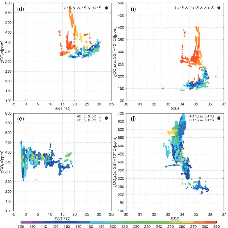
Figure 3. Relationships between xCO2s and SST (left column) or SSS (right column) in five regions of the Pacific Ocean: (a) and (f), NP/A; (b) and (g), NP/T; (c) and (h), EQ; (d) and (i), SP/T;
(e) and (j), SP/A. The labels “Positive” or “Negative” indicate the signs of the regression coefficients between xCO2s and SST or SSS.
- 10 - 3.2.2. The equatorial region (EQ)
The easterly trade winds cause equatorial upwelling. This upwelling brings cold and carbon-rich water from deeper layers to the surface. In the equatorial region, SST and xCO2s are negatively correlated and this relationship varies seasonally and annually. Cosca et al. (2003) and Feely et al. (2006) used this relationship to derive seasonal and inter-annual equations for estimates of pCO2s. In contrast, Nakadate and Ishii (2007) and Ishii et al. (2009) used SSS to divide the equatorial region into the warm pool region and the upwelling region and derived two equations to calculate xCO2s. In this region ENSO determines the strength of upwelling and the wind patterns, which cause inter-annual variation of CO2 flux (Cosca et al., 2003; Feely et al., 2006; Nakadate and Ishii, 2007; Ishii et al., 2009).
In the equatorial upwelling region, we found a negative linear relationship between SST and xCO2s that varies seasonally, as reported by Cosca et al. (2003) and Feely et al. (2006) (blue oval in Fig. 3c). The relationship between SSS and n-xCO2s is a quadric convex distribution and n-xCO2s reaches a peak at SSS = 35 (blue oval in Fig. 3h).
The warm-pool region spreads to the west of the upwelling region where there is a positive linear relationship between SST and xCO2s. The relationship between SSS and n-xCO2s is not clear in this region (red oval in Fig. 3c and 3h). East of the upwelling region, SSS and xCO2s are relatively low (green oval in Fig. 3c and 3h). A positive relationship between SSS and n-xCO2s is seen in this region where SSS is above 34.
W) 120 of (east 34
120°W) and
160°W (between
40 160 35
W) 160 of west ( 35
SSSbnd lon (5)
where ‘lon’ indicates longitude in degrees west. The area where SSS ≥ SSSbnd is classified as the upwelling region (Region H) and the region where SSS < SSSbnd contains the other two sub-regions. The area where SSS < SSSbnd is divided into two smaller regions at 140°W. The area west of 140°W is regarded as the warm pool region (Region G) and east of 140°W is the low salinity region (Region I).
Eq. 6 below is the empirical formula for the distribution of xCO2s in the equatorial region. We used a quadratic expression because of the quadric convex relationship between SSS and n-xCO2s in the upwelling region (blue oval in Fig. 3h). A sine-function term for the month (“Mn” in Eq. 6; 1 to 12 for January through December, respectively) is added to the equation only in the upwelling region to express the seasonal variation.
sin 2 12
s
CO2 25 35 252 352 25 35 2000 Mn i
h Yr g S T f S e T d S c T b
a (6)
x
On the basis of these observations, we divided the equatorial region into three sub-regions: the warm pool region (G), the upwelling region (H) and the low salinity region (I). The geographic distribution of these three sub-regions varies with time depending on the distribution of SSS. The boundary between the upwelling region and the other two regions is defined by the following relationship:
- 11 -
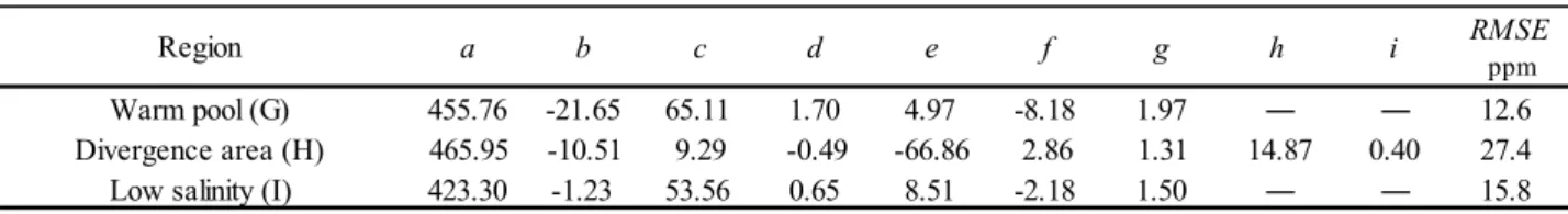
The coefficients and root mean square errors (RMSEs) for each region are listed in Table 2.
Table 2. Coefficients and RMSEs for the multiple regression Eq. 5 for each sub-region in the equatorial Pacific (EQ). Letters after sub-region names correspond to the region codes in Figure 1.
RMSE ppm
Warm pool (G) 455.76 -21.65 65.11 1.70 4.97 -8.18 1.97 ― ― 12.6
Divergence area (H) 465.95 -10.51 9.29 -0.49 -66.86 2.86 1.31 14.87 0.40 27.4
Low salinity (I) 423.30 -1.23 53.56 0.65 8.51 -2.18 1.50 ― ― 15.8
Region a b c d e f g h i
3.2.3. The subpolar regions
In the subpolar regions, strong vertical mixing supplies inorganic carbon from deep cold waters each winter. The increase in xCO2s by vertical mixing exceeds xCO2s reduction by seasonal cooling. There is a negative relationship between SST and xCO2s in this region (Takahashi et al., 1993; Park et al., 2006).
In addition, phytoplankton consumes inorganic carbon in spring, with more consumption in the western North Pacific. To estimate the carbon reduction, previous studies have used Chl-a levels measured by remote sensing (Ono et al., 2004; Sarma et al., 2006; Chierici et al., 2009). In general, Chl-a is negatively correlated with xCO2s because more carbon is consumed when more Chl-a is observed.
3.2.3.a The North Pacific (NP/A)
There is a positive linear relationship between SST and xCO2s in the region of the subarctic North Pacific where SST ≥ 16 °C, as was also seen in the subtropical region (red oval in Fig. 3a). In this region, nutrients are exhausted and xCO2s mainly varies from the thermodynamic effect. The intercept of the linear regression at 25 °C gradually increases toward the east. There is a negative relationship between SSS and n-xCO2s in this region (red oval in Fig. 3f; referred as ‘the northern subtropical region’ (defined later)), with SSS increasing from west to east.
In the open ocean where SST < 16 °C and west of 160°E, there is a negative linear relationship between SST and xCO2s (blue and orange ovals in Fig. 3a) and no significant relationship between SSS and n-xCO2s.
In the region where 5 °C ≤ SST < 16 °C, the slope of the linear regression between SST and xCO2s in summer (from July to September) is smaller than that in other seasons. This shows that the balance between factors that determine xCO2s varies seasonally.
The slope of linear regression between SST and xCO2s gets steeper in the region where SST < 5 °C because CO2-rich water is supplied from deeper waters by the western subarctic circulation and vertical mixing.
In the Oyashio region and the region where SST < 16 °C, xCO2s is very low and there is no clear relationship between SST and xCO2s because phytoplankton blooms consume most of the CO2 (green oval in Fig. 3a).
Based on these observations, we divided the subarctic region into three smaller regions: the northern subtropical region (SST ≥ 16 °C; Region C), the southern subarctic region (5 °C ≤ SST < 16 °C;
- 12 -
Region B) and the northern subarctic region (SST < 5 °C; Region A). We produced regression equations for each sub-region. Two equations are needed for the southern subarctic region to account for seasonal differences between summer and other seasons. The equation for Region A (SST < 5 °C) is as follows:
2000 10
2s 288.62 14.21 1.40
CO T Yr (±24.6) (7).
The equation for Region B (Oct–Jun; 5 °C ≤ SST < 16 °C) is as follows:
2000 10
2s 345.42 3.10 1.40
CO T Yr (±15.1) (8),
and for Jul–Sep (5 °C ≤ SST < 16 °C) as follows:
2000 10
2s 358.73 1.85 1.40
CO T Yr (±21.2) (9).
For Region C (SST ≥ 16 °C), the equation is as follows:
2000 160
33 10
2s 248.10 9.86 12.78 0.76 1.40
CO T S Lon Yr (±15.1) (10),
where T10, S33, Lon160 and Yr2000 are defined as [SST − 10], [SSS − 33], [longitude (°E) − 160] and [year − 2000], respectively.
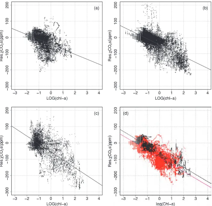
It is also necessary to consider the biological activity in the regions off the Sanriku coast in Japan and around the Aleutian Islands (Ono et al., 2004; Sarma et al., 2006; Chierici et al., 2009). Chierici et al.
(2009) reported that the use of log-transformed Chl-a data significantly improves the fit of the multiple regressions for estimating pCO2s.
We compared the logarithm of Chl-a with the residual error between estimated and observed xCO2s (Fig. 4a–4c) and found negative linear relationships. We generated linear regression equations to estimate the biological consumption of CO2 (Bio) in each region.
Region A (SST < 5 °C): Bio55.1148.47ln[Chl-a] (± 50.3) (11)
Region B (Oct–Jun ; 5 °C ≤ SST < 16 °C):Bio44.8536.27ln[Chl-a] (± 29.3) (12)
Region B (Jul–Sep ; 5 °C ≤ SST < 16 °C):Bio42.9930.34ln[Chl-a] (± 39.8) (13)
Negative values for Bio indicate that xCO2s is overestimated using SST and SSS and that CO2 is consumed by biological activity. For the regions west of 160°E or north of 50°N only, where there is high biological activity, if Eq. 11–13 yield negative values for Bio, then the value for Bio is respectively added to xCO2s as estimated by Eq. 7–9. The introduction of the Bio term reduces the average bias of the estimates to
±10 ppm.
x
x
x
x
- 13 -
Figure 4. Relationships between the residual error between estimated and observed xCO2s and the logarithm of chlorophyll-a concentrations determined by remote sensing from satellite. (a) The southern subarctic region within NP/A (summer: July–September), (b) the southern subarctic region within NP/A (winter: October–June), (c) the northern subarctic region within NP/A, (d) SST < 3℃ region within SP/A (black, October–December; red, January–April). Lines and shade areas are regression lines and 95% confidence intervals, respectively.
3.2.3.b. The South Pacific (SP/A)
The relationship between SST and xCO2s changes at SST = 16 °C in the western portion of the South Pacific (140°E) and at SST = 10 °C in the east (70°W). This relationship is negative in the region of lower SSTs (orange oval in Fig. 3e) and positive at higher SSTs (red oval in Fig. 3e). In the region where SST < 3 °C, there is substantial biological consumption and no evident relationship between SST and xCO2s when sea-ice melts in austral summer (green oval in Fig. 3e).
We divided the subantarctic South Pacific into three smaller regions using the following criteria:
- 14 -
1. Because the rates of increase of xCO2s differ between the northern region (north of 55°S) and the southern region (south of 55°S), as discussed in Section 3.1, the subantarctic South Pacific is divided into two regions at 55°S.
2. The northern region is divided into two regions by a boundary SST (SSTbnd), defined as follows:
E) 140 ) E ( 150(
16 6
longitude
SSTbnd (14)
The part of the northern region where SST < SSTbnd is called the northern subantarctic region (M) and where SST ≥ SSTbnd is the southern subtropical region (L).
3. The southern region (south of 55°S) is called the southern subantarctic region (N).
The relationship between SSS and n-xCO2s is negative in the southern subtropical region. We produced multiple regressions Eq. 15–17 to calculate xCO2s in the three regions using SST and SSS. For Region L (north of 55°S and SST ≥ SSTbnd), the equation is as follows:
2000 180
33
2s 322.90 2.23 10.24 0.44 1.30
CO T S Lon Yr (±14.3) (15),
for Region M (north of 55°S and SST < SSTbnd):
2000 33
2s 399.97 6.62 11.50 1.30
CO T S Yr (±15.0) (16),
and for Region N (south of 55°S):
2000 33
2s 363.06 0.44 4.19 2.20
CO T S Yr (±13.5) (17),
where Lon180 is the longitude (°E) minus 180.
In the Antarctic region (SST < 3°C), we introduce the Bio term to express biological consumption as in the subarctic region in the North Pacific. We produced two linear regression equations because the intercept of the regression between the logarithm of Chl-a concentration and the residual error of xCO2s from Eq. 17 changes between spring/early summer (October–December; black symbols in Fig. 4d) and late summer/autumn (January–April; red symbols in Fig. 4d). In areas where Bio was negative, as estimated by Eq. 18 and 19, it was added to xCO2s:
Region N (Oct–Dec), Bio61.0543.94ln[Chl-a] (±23.8) (18)
Region N (Jan–Apr), Bio87.5643.49ln[Chl-a] (±32.0) (19) x
x
x
- 15 -
4. pCO2s estimation and associated error
We estimated monthly pCO2s in a 1° × 1° grid from 1985 through 2009 by using the grid data described in Section 2 and the empirical equations introduced in Section 3. Data for Chl-a by remote sensing have been available only since 1998. For pCO2s estimates before 1998 we used the climatological Chl-a, which is the average of monthly remote sensing data sets from 1998 through 2009.
We generated time series of monthly pCO2s and pCO2a averaged in the five regions since 1985 (Fig.
5). The estimates for 25 years agree with observations very well in the five regions. For example, our method adequately reproduced the drastic decrease in pCO2s in the equatorial region during 1997/1998 El Niño. The method also estimates pCO2s in subarctic regions where large seasonal variations in pCO2s occur because of biological consumption and vertical mixing.
We determined the annual mean bias and RMSE between pCO2s estimates and observations in each region over 25 years. For error estimation in 2007 and 2008, we also used the latest LDEO Database V2008 (Takahashi et al., 2009a). The mean biases in all regions are small, ranging from −10 to +10 µatm (Fig. 6). The RMSE in the subarctic regions and the equatorial region (approximately 30 µatm) is relatively larger than that in the subtropical regions (about 20 µatm).
We used monthly mean SST, SSS and Chl-a data to estimate monthly pCO2s fields. These data sets represent a different time-scale than observational data, which are instantaneous values. This difference in
Figure 5.
Time series of pCO2s (solid lines, estimated; circles, observed) and pCO2a (broken line).
(a) NP/A (45°N-50°N, 150°E-160°E);
(b) NP/T (15°N-20°N, 130°E-140°E);
(c) EQ (5°S-EQ, 120°W-110°W); (d) SP/T (20°S-15°S, 180°-170°W); and (e) SP/A (65°S–60°S, 180°–170°W).
Regions (a)–(e) are shown in (f).
Error bars (pCO2s observations) and shaded areas (pCO2s estimates) show standard deviations (1σ).
- 16 - time-scale causes some error in pCO2s estimation.
The differences between estimates and observations in the subtropical and warm-pool regions are smaller than those in the equatorial upwelling region and subarctic regions. This is because the estimation errors in subtropical and equatorial warm-pool regions, where pCO2s varies mainly because of the thermodynamic effect, are based almost entirely on SST data errors.
In the equatorial region, the boundaries between the upwelling region, the low salinity region and the warm-pool region are determined by monthly SSS data, but these boundaries actually shift over shorter time scales. This time lag in region division increases the estimation error in the equatorial region.
In the subpolar regions, monthly Chl-a fields are used for pCO2s estimation. pCO2s is very sensitive to Chl-a levels, which vary widely over short time intervals. Furthermore, climatological Chl-a was used for pCO2s estimates before 1998. These factors increase RMSEs in the subpolar regions.
Figure 6. Annual mean biases (a) and annual RMSE (root mean square error) (b) between estimated and observed pCO2s in each region. Bias is defined as (pCO2s [estimated] – pCO
2s
[observed])/n, and RMSE is defined as (pCO2s [estimated] – pCO2s [observed])2/(n−1). n is the number of data.
- 17 - 5. Net sea-air CO2 flux estimation
5.1. Computational method for estimating CO2 flux
The net sea-air CO2 flux (FCO2) can be estimated using Eq. 18:
2
CO CO
2 K p
F
(18)
In this equation, K is the gas transfer coefficient and pCO2 is the difference in pCO2 between sea and air (=pCO2s − pCO2a). K is the product of the gas transfer velocity (k) and the solubility of CO2 in seawater (L).
k is calculated by the method of Wanninkhof (1992), which uses monthly U10 values. L is based on the equation of Weiss (1974).
5.2. Seasonal average and variation of CO2 flux
The 25-year mean monthly CO2 flux maps for February, May, August and November show the typical horizontal distribution of the CO2 flux from 1985 to 2009 (Fig. 7). In the equatorial region, pCO2s is larger than pCO2a throughout the year, and this region is a major CO2 source for the atmosphere. This is because of the inorganic carbon supplied from the deeper oceanic layers through equatorial upwelling.
In the subtropical region, because biological CO2 consumption is low and the mixed layer is shallow, pCO2s varies with SST because of the thermodynamic effect. pCO2s is therefore the highest when SST is the highest during summer in each hemisphere and CO2 uptake in summer is less than in winter. In the North Pacific, pCO2s in the western region and the coastal region off California is higher than in the other regions. The western region is affected by the Kuroshio and the coastal region off California is influenced by subarctic seawater rich in carbon. The region east of Hawaii is located in the marginal zone between subtropical warm water and subarctic cold water rich in carbon and nutrients; the subtropical water is cooled by the subarctic water and carbon is consumed through biological activity. As a result, pCO2s in this region is relatively low. However, pCO2s increases from west to east in the South Pacific. The coastal region off Peru in particular is influenced by coastal upwelling and emits CO2 to the atmosphere.
In the subpolar regions, pCO2s is the highest in winter because vertical mixing supplies carbon-rich water from lower layers. In the region east of Japan and in the antarctic region, pCO2s decreases from spring to summer when phytoplankton consumes CO2.
The marginal zone between the subtropical and subarctic regions in the Pacific is a major CO2 sink.
Because SST decreases and seasonal wind intensifies in winter, pCO2s decreases from the thermodynamic effect and the gas transfer coefficient increases. As a result, CO2 uptake is highest in winter.
Larger standard deviations of CO2 flux are seen around the equatorial region and the boundary between the subtropical and subpolar regions (Fig. 8). pCO2s in the equatorial region is affected by ENSO, as mentioned in Section 4. The ENSO cycle affects pCO2s and wind patterns, causing variations in the CO2 flux.
In the North Pacific boundary region, SST and SLP variations caused by the PDO are predominant. The PDO could affect pCO2s or U10 (and the gas transfer velocity) through anomalies in SST and SLP.
- 18 -
Figure 7. Monthly mean CO2 flux maps for February, May, August and November. The color scale shows the level of CO2 source or sink.
Figure 8. Standard deviations of monthly CO2 flux (mol m–2 yr–1) in February, May, August and November.
- 19 - 5.3. Time series of area-integrated CO2 flux
We calculated the area-integrated monthly and annual CO2 flux from 1985 through 2009 (Fig. 9).
In the equatorial region, CO2 outgassing varies with ENSO. CO2 emission decreases during El Niño periods (ENSO warm phase) and increases for La Niña periods (ENSO cold phase). For the 1997/1998 El Niño period in particular, CO2 emission was 70% of that during normal periods.
In contrast, seasonal variation predominates in the subtropical regions, and CO2 uptake decreases in summer and increases in winter. The amplitude of the variation in CO2 flux is greater in the northern hemisphere than in the southern. This reflects the larger seasonal SST amplitude and more severe winter winds in the northern hemisphere.
Figure 9. Time series of regional CO2 flux (PgC yr–1) for the Pacific Ocean. Lines and boxes show monthly and annual CO2 flux, respectively. Shading indicates ENSO events: dark grey, El-Niño; light grey, La-Niña.
As in the subtropical regions, there is seasonal variation in the subarctic region as well. Unlike the subtropical regions, the CO2 flux in the subarctic region is at a minimum in spring due to biological uptake of CO2. There is seasonal variation in CO2 flux in the subantarctic region, with a maximum uptake by the sea in austral summer and a minimum uptake in austral winter. This is because the amount of inorganic carbon supplied by vertical mixing is small and biological uptake increases in austral summer.
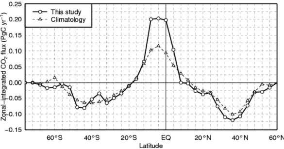
- 20 - 5.4. Comparison with the climatological CO2 flux
We compared the meridional distribution of the CO2 flux in 2000 determined in this study with the climatological CO2 flux for the reference year 2000 as reported by Takahashi et al. (2009b) (Fig. 10). The results of this study correspond qualitatively with the climatology. However in the equatorial region the flux estimated in this study is double the climatological flux estimate.
Table 3 presents the comparison between the flux determined in this study and the climatological flux estimate in each zonal band. The absolute values from this study are larger than those of the climatology in all zonal bands. In this study we used different U10 analysis data and a different equation for the gas transfer coefficient than used for the climatology data. As a result, the gas transfer coefficients in this study are from about 1.5 to 2 times those of the climatology.
Because a La Niña event continued until the spring of 2000, the pCO2s values in this study, which reflect the real-time oceanic conditions, are larger than the climatological pCO2s in the equatorial region (Fig.
11). The difference between the CO2 flux estimates results from the difference in gas transfer coefficient and Figure 10. Meridional distribution of the zonally-integrated CO2 flux (PgC yr–1) in 2000 from this study
(solid line) and the climatological CO2 flux in the reference year 2000 from Takahashi et al.
(2009b) (dashed line).
In 2000 (PgC yr-1)
Average 1985-2009 (PgC yr-1)
N. of 50°N –0.06 –0.06±0.01 –0.03
14°N-50°N –0.64 –0.70±0.05 –0.50
14°S-14°N +0.77 +0.62±0.10 +0.48
50°S-14°S –0.42 –0.46±0.08 –0.41
Sum. –0.34 –0.59±0.14 –0.46
Zone
This study Takahashi et al. (2009b) (PgC yr-1) Table 3. Comparison between the CO2 fluxes estimated in this
study and the climatological CO2 flux in each zonal band. The gas transfer coefficient used in this study is from the equation of Wanninkhof (1992). Positive and negative CO2 fluxes refer to sea-to-air or air-to-sea transfers of CO2, respectively. The column “The average values for 1985–2009” is the average and standard deviation of the annual mean CO2 fluxes between 1985 and 2009.
- 21 - the La Niña event.
In the Pacific north of 50°S, the mean flux from 1985 through 2009 estimated in this study is −0.59 PgC yr–1; the flux estimate for 2000 is −0.34 PgC yr–1 and the climatological flux in the reference year 2000 is −0.46 PgC yr–1. The estimated annual CO2 flux in 2000 from this study is smaller uptake than the climatological estimate because of the influence of La Niña. The mean annual flux from this study is larger uptake than the climatological flux estimate because of the difference in the gas transfer coefficients.
The surface of the Pacific Ocean accounts about 46% of the ocean surface worldwide.
However, the average CO2 uptake in the Pacific as estimated in this study is about 32% of the total absorption by the Global Ocean (2.2 PgC yr–1; IPCC, 2007). The proportional CO2 uptake in the Pacific Ocean is smaller than the proportional area because of the Pacific equatorial region, which is the area of greatest CO2 release in the world.
5.5. Effects of gas transfer coefficient equations on CO2 flux
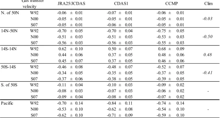
We used the formula of Wanninkhof (1992; hereafter “W92”) to estimate CO2 flux. In other recent studies, other formulas have been proposed, such as those of Nightingale et al. (2000; hereafter “N00”) and Sweeney et al. (2007; hereafter “S07”). We compared the CO2 fluxes estimated using gas transfer coefficients calculated using these three formulas. The results of this comparison are summarized in Table 4.
Absolute value of annual mean CO2 flux estimates based on N00 using JRA25/JCDAS wind speed fields were the lowest and those using W92 were the highest. In each region, the difference between gas transfer coefficients is 15–20%. This difference is comparable to the uncertainty in the gas transfer coefficients of about 30% (Sweeney et al., 2007).
5.6. Effect of wind speed on CO2 flux
To calculate gas transfer coefficients we used not only the wind velocity fields from JRA25/JCDAS but also those from National Centers for Environmental Prediction / National Center for Atmospheric Research (NCEP/NCAR) Reanalysis I (Kalnay et al., 1996; hereinafter CDAS1) and from a Figure 11. Mean difference between the pCO2s values
in 2000 estimated in this study and the climatological pCO2s values (Takahashi et al., 2009b). The difference is defined as the value from this study minus the climatological value.
- 22 -
cross-calibrated, multi-platform (CCMP), multi-instrument ocean surface wind velocity data set (Ardizzone et al., 2009). We used SLP fields from JRA25/JCDAS because the mean SLP difference between JRA25/JCDAS and CDAS1 is about 1 hPa and this results in a difference in pCO2s of only 0.1% (0.4 µatm).
The effect of the SLP difference is less than the pCO2s estimation error of −10 to +10 µatm.
In Table 4, we summarize the annual regional CO2 flux as estimated using three different types of U10 data. Except for the equatorial region (14°S–14°N), the CO2 flux estimates agree with each other. In the equatorial region, CO2 emission based on CDAS1 is the smallest among the three wind velocity fields. For example, the difference in CO2 flux estimates based on the JRA25/JCDAS and CDAS1 U10 fields using the W92 equation is about 20% (0.12 PgC yr–1). This is because the U10 of CDAS1 is 10% weaker than that of JRA25/JCDAS due to the differences of models and assimilated datasets. When the gap between U10 values is 10%, that between gas transfer coefficients accounts for about 20% of the difference because the gas transfer coefficient is proportional to the square of U10. For the entire Pacific Ocean, estimates using JRA25/JCDAS show lower CO2 uptake than those using CDAS1 because of higher CO2 emission in the equatorial region.
Table 4. Comparison of different estimates of the CO2 flux (PgC yr–1) for each zonal band using equations for gas transfer coefficients from three sources — Wanninkhof (1992; W92), Nightingale et al. (2000; N00) and Sweeney et al. (2007; S07) — and U10 fields from JRA25/JCDAS, NCEP/NCAR Reanalysis I, and a cross-calibrated, multi-platform (CCMP) dataset. Values for CO2 flux are means and standard deviations from 1985 through 2009 (1990–2009 for CCMP).
as transfer
velocity Clim
N. of 50N W92 -0.06 ± 0.01 -0.07 ± 0.01 -0.06 ± 0.01
N00 -0.05 ± 0.01 -0.05 ± 0.01 -0.05 ± 0.01
S07 -0.05 ± 0.01 -0.06 ± 0.01 -0.05 ± 0.01
14N-50N W92 -0.70 ± 0.05 -0.70 ± 0.04 -0.75 ± 0.05
N00 -0.51 ± 0.03 -0.51 ± 0.03 -0.53 ± 0.03
S07 -0.56 ± 0.03 -0.56 ± 0.03 -0.55 ± 0.03
14S-14N W92 0.62 ± 0.10 0.50 ± 0.07 0.68 ± 0.09
N00 0.44 ± 0.06 0.37 ± 0.05 0.48 ± 0.06
S07 0.45 ± 0.07 0.37 ± 0.05 0.46 ± 0.06
50S-14S W92 -0.46 ± 0.08 -0.48 ± 0.07 -0.52 ± 0.07
N00 -0.34 ± 0.05 -0.35 ± 0.05 -0.37 ± 0.05
S07 -0.37 ± 0.06 -0.38 ± 0.05 -0.39 ± 0.05
S. of 50S W92 -0.11 ± 0.04 -0.10 ± 0.03 -0.09 ± 0.02
N00 -0.08 ± 0.03 -0.07 ± 0.03 -0.06 ± 0.02
S07 -0.09 ± 0.04 -0.08 ± 0.03 -0.07 ± 0.02
Pacific W92 -0.70 ± 0.14 -0.84 ± 0.11 -0.74 ± 0.14
N00 -0.53 ± 0.10 -0.62 ± 0.08 -0.54 ± 0.10
S07 -0.62 ± 0.10 -0.71 ± 0.09 -0.59 ± 0.10
JRA25/JCDAS CDAS1
-
- CCMP
-0.03
-0.50
0.48
-0.41 G
6. Summary and conclusions
We developed an empirical method to estimate monthly pCO2s and sea-air CO2 flux over the Pacific since 1985 using the LDEO database V1.0 (Takahashi et al., 2008) of global pCO2s observations.
First, we determined the long-term trend of pCO2s. Second, we analyzed regional and seasonal variations of pCO2s. We divided the Pacific Ocean into 14 regions and derived multiple regression equations for estimating monthly pCO2s for each region incorporating data for SST, SSS and Chl-a. Previously it had been difficult to reproduce pCO2s in the subpolar regions where there are spring blooms and high net biological consumption of inorganic carbon, but the bias in the estimates was significantly reduced by including Chl-a data in the analysis. Mean bias of estimated pCO2s in each region ranged from –10 to +10 µatm.
The estimated mean annual CO2 flux in the Pacific Ocean is −0.70 ± 0.14 PgC yr–1 (negative value indicates uptake by the ocean) for the period from 1985 to 2009. The CO2 flux varies seasonally and inter-annually. While there is CO2 emission throughout the year in the equatorial region, there is strong CO2 uptake along the mid-latitudes in winter. We found that CO2 flux in the equatorial region varies largely with ENSO. In particular, the CO2 emission decreased by 0.2 PgC yr–1 during the 1997/1998 El Nino event. The region included in this study is about 46% of the global ocean. To further understand the global carbon cycle, it will be necessary to investigate whether the empirical method developed in this study can be applied to the Atlantic and Indian oceans to expand the region of CO2 flux estimation.
There is a significant uncertainty remaining in the CO2 flux estimates. The different gas transfer coefficient equations used in this study resulted in differences of 15% to 20% in estimated fluxes. The CO2 emission in the equatorial region, when evaluated using the wind-speed product from the JRA25/JCDAS reanalysis, is about 0.12 PgC yr–1 (20%) higher than that estimated using CDAS1. The CO2 flux estimates in the other regions are consistent between reanalysis data sets.
To reduce the uncertainty in CO2 flux estimates, it will be necessary to continue investigations into better wind-speed analysis and gas transfer coefficients. There are plans to update the global pCO2s database annually with the accumulated pCO2s observation data. Therefore, there should be a continuous review of the equations and the regional divisions used for pCO2s estimation to reduce uncertainties where the data are sparse. It is important to use observations to monitor inter-annual variations and long-term trends of pCO2s.
Furthermore, it is important to compare CO2 flux as estimated using other approaches such as atmospheric CO2 inversion, forward ocean carbon cycle modeling, and ocean carbon inversion.
Discrepancies in the estimates from these methods must be reduced to better understand the carbon cycle and to improve projections of global warming.
- 23 -