On Constructive Linear-Time Temporal Logic

or with entcsmacro.sty for your meeting. Both can be found at the ENTCS Macro Home Page.

On Constructive Linear-Time Temporal Logic

Kensuke Kojima ¹ and Atsushi Igarashi ²

Graduate School of Informatics Kyoto University

Kyoto, Japan

Abstract

In this paper we study a version of constructive linear-time temporal logic (LTL) with the “next” temporal operator. The logic is originally due to Davies, who has shown that the proof system of the logic corre- sponds to a type system for binding-time analysis via the Curry-Howard isomorphism. However, he did not investigate the logic itself in detail; he has proved only that the logic augmented with negation and classical reasoning is equivalent to (the “next” fragment of) the standard formulation of classical linear-time temporal logic. We give natural deduction and Kripke semantics for constructive LTL with conjunction and disjunction, and prove soundness and completeness. Distributivity of the “next” operator over disjunction

“(A ∨ B) ⊃ A ∨ B” is rejected from a computational viewpoint. We also give a formalization by sequent calculus and its cut-elimination procedure.

Keywords: constructive linear-time temporal logic, Kripke semantics, sequent calculus, cut elimination

1 Introduction

Temporal logic is a family of (modal) logics in which the truth of propositions may depend on time, and is useful to describe various properties of state transition systems. Linear-time temporal logic (LTL, for short), which is used to reason about properties of a fixed execution path of a system, is temporal logic in which each time has a unique time that follows it.

Davies [3] pointed out that a proof system of LTL can be related to a type system of (multi-level) binding-time analysis, which is used in offline partial evaluation [8]

to determine which part of a program can be computed at specialization-time and which is residualized. He defined a natural deduction system for a constructive LTL with only the “next” operator and implication, derived via the Curry-Howard isomorphism a typed λ-calculus λ , which was formally shown to be equivalent to a type system of multi-level binding-time analysis by Gl¨ uck and Jørgensen [6].

According to this correspondence, a formula A, which means that A holds at the next time, is interpreted as a type of (residual) code of type A; introduction and

1

Email: [email protected]

2

Email: [email protected]

elimination rules of are as Lisp-like quasiquotation and unquote, respectively.

As a result, λ terms can be considered as program-generating programs, such as parser generators or generating extensions, which manipulate code fragments by the quasiquotation mechanism. For example, a parser generator would have a type like parser spec → (string → syntax tree). Unfortunately, Davies did not investigate his system in detail, from a logical point of view: he proved only that his system augmented with negation and classical reasoning is equivalent to the classical LTL, even though the logic can be considered a constructive version of LTL.

In this paper we study logical aspects of constructive propositional LTL based on Davies’ formalization. Davies’ original system is an implicational fragment, but we also consider conjunction and disjunction. ³ Our contributions are (1) to give a Kripke semantics and a complete proof system for constructive LTL and (2) to give another formalization by sequent calculus in which cut elimination holds.

Intuitionistic versions of LTL have been already considered in the literature [9,4].

However, the LTL presented in this paper is motivated by the type-theoretic inter- pretation of A as a type of quoted code, which distinguishes our approach from others. In fact, our version of LTL is not equivalent to the intuitionistic LTLs previously considered in that the “distributivity law” (A ∨ B) ⊃ A ∨ B is not admitted in our logic, while (to our knowledge) it is admitted in the other formalizations. The reason we disallow this law will be discussed later.

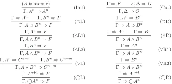
The organization of the rest of this paper is as follows. In Section 2, we discuss an implicational fragment: we first review the natural deduction by Davies, give a Kripke semantics, obtained by a natural extension of that of the classical LTL, and finally prove soundness and completeness of the proof system. We also discuss that, unfortunately, a straightforward extension of the semantics to disjunction is not suitable for our interpretation of disjunction. In Section 3 we extend the logic with conjunction and disjunction. We give another Kripke semantics, which does not admit the distributivity law mentioned above, and prove soundness and completeness of the proof system. In Section 4 we define a sequent calculus LJ , which is equivalent to the natural deduction, with its cut elimination procedure.

Finally, we give concluding remarks in Section 5.

2 Implicational Fragment

In this section, we first recall the natural deduction system by Davies and some of its properties, define a Kripke semantics for it, and prove completeness of Davies’

system.

2.1 Results by Davies

The temporal logic Davies considered contains only (“next” operator) and ⊃ (intuitionistic implication), so the language we consider in this section is constructed from propositional variables using ⊃ and .

3

Precisely speaking, Davies extended λ

with pairing and natural numbers, but did not consider conjunc-

tion or disjunction in his logic.

Γ, A ⁿ ⊢ A ⁿ (Axiom) Γ ⊢ A ⊃ B ⁿ Γ ⊢ A ⁿ

Γ ⊢ B ⁿ (⊃E)

Γ ⊢ A ⁿ

Γ ⊢ A ⁿ⁺¹ (E)

Γ, A ⁿ ⊢ B ⁿ

Γ ⊢ A ⊃ B ⁿ (⊃I)

Γ ⊢ A ⁿ⁺¹

Γ ⊢ A ⁿ (I)

Fig. 1. Derivation Rules of Davies’ System.

A judgment in his system takes the form A ⁿ ₁

, . . . , A ⁿ _k

⊢ B ^m

where A i , B are formulas and n i , m are natural numbers; it is read “B holds at time m under the assumption that A i holds at time n i (for i = 1, . . . , k)”. In what follows, we use A, B, C, D for formulas, k, l, m, n for natural numbers, F, G for annotated formulas (i.e. formulas with time annotation), and Γ, ∆ for sets of annotated formulas. We consider the left-hand side of a judgment a set.

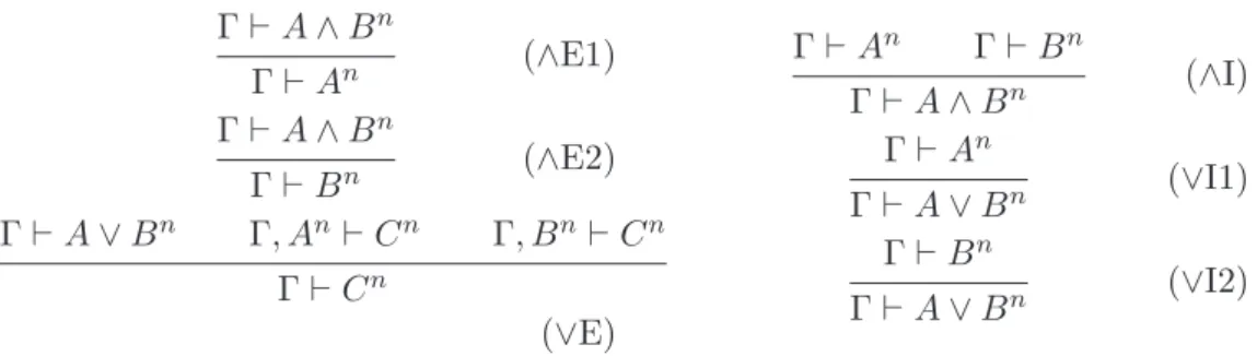
Inference rules of Davies’ system are listed in Fig. 1. The rules ⊃I, ⊃E, and Axiom are standard. The other two, the introduction and elimination rules for operator, state that A holds at time n + 1 if and only if A holds at time n. This is quite natural since A means that “A holds at the next time.”

To show that operator in this system is indeed the “next” operator in linear- time temporal logic, Davies compared his system with L , a well-known Hilbert- style proof system of the fragment of classical linear-time temporal logic consisting of only implication, negation and next operators. The axiomatization is given by Stirling, who also proved that L is sound and complete for the standard seman- tics [12]. The axioms and rules of L are as follows:

Axioms ^• any classical tautology instance

• ¬A ⊃ ¬ A

• ¬ A ⊃ ¬A

• (A ⊃ B) ⊃ A ⊃ B Rules ^• if A ⊃ B and A then B

• if A then A

Davies proved that his system extended by negation and classical reasoning is equiv- alent to L in the following sense [3]:

Proposition 2.1 A judgment A ⁿ ₁

, . . . , A ⁿ _k

⊢ B ^m is provable in the extended sys- tem if and only if ⁿ

A ₁ ⊃ . . . ⊃ ⁿ

A k ⊃ ^m B has a proof in L . In particular,

· ⊢ A ⁰ is provable if and only if A is a theorem of L .

2.2 Kripke Semantics via Functional Frames

Before discussing the semantics of the implicational fragment, we briefly explain

how the usual classical semantics is given in terms of Kripke semantics. Kripke

frames we consider are functional, in the sense that the accessibility relation R on

possible worlds is a map. ⁴ This condition guarantees that, in a functional frame, the next state of a given state is uniquely determined, hence justifying “linear time”.

To give a semantics of constructive LTL, we follow the previous researches on Kripke-style models of intuitionistic modal logics [1,14,2] and augment functional frames by another accessibility relation ≤. This additional accessibility represents the “constructive” counterpart, as in the standard semantics of intuitionistic logic.

Definition 2.2 An intuitionistic functional frame is a triple hW, ≤, Ri of a nonempty set W , a preorder ≤ on W and a map R from W to W such that ≤ ◦ R = R ◦ ≤ holds. Here ◦ stands for a composition of binary relations defined by x R ◦ S y ⇐⇒

∃z.(x R z S y).

This notion is an extension of classical functional frames: if ≤ is the diagonal relation (that is, x ≤ y if and only if x = y) in this definition, the frame hW, ≤, Ri can be identified with a classical functional frame hW, Ri. Hereafter, we simply say functional frame when no confusion arises.

Using functional frames we can define a satisfaction relation on formulas.

Definition 2.3 Let hW, ≤, Ri be a functional frame and | = be a binary relation between W and the set of propositional variables such that w ≤ w ^′ and w | = p imply w ^′ | = p. We extend | = to formulas by induction with

• w | = A ⊃ B ⇐⇒ if w ≤ w ^′ and w ^′ | = A then w ^′ | = B, and

• w | = A ⇐⇒ if w R w ^′ then w ^′ | = A.

We also write w | = A ⁿ for w | = ⁿ A.

This definition is one of the standard semantics of intuitionistic modal logics pre- viously considered [14]. As is easily verified by induction on the construction of formulas, this semantics satisfies the monotonicity condition.

Lemma 2.4 If w ≤ w ^′ and w | = A, then w ^′ | = A.

It is not very difficult to see that the Davies’ system is sound and complete for this semantics. Soundness is proved by straightforward induction on the derivation.

Completeness is proved by constructing a functional frame in which validity and provability coincide. We sketch the proof below.

For a set T of formulas, we write ⁻¹ T for the set {A | A ∈ T } and T for {A | A ∈ T }. Take the set of all theories as W , let ≤ be a set-inclusion, and R the map which sends each theory T to the theory ⁻¹ T . First we show that this defines a functional frame.

Lemma 2.5 The canonical frame hW, ≤, Ri above is indeed functional.

Proof. Among conditions of being a functional frame, the only nontrivial one is R ◦ ≤ ⊆ ≤ ◦ R. To show this, take theories T and S with ⁻¹ T ⊆ S (i.e. T (R ◦ ≤) S), and let U be the smallest theory containing T and S. We are going to show that U satisfies T ≤ U R S, i.e. T ⊆ U and ⁻¹ U = S.

Clearly, T ⊆ U holds by definition. It is also easy to see that S ⊆ ⁻¹ U : if

4

The term “functional” is, to our knowledge, first used by Segerberg [11], but not in context of semantics

of LTL.

A ∈ S, then A ∈ S ⊆ U , and from this A ∈ ⁻¹ U follows. For the converse, let A be a formula in ⁻¹ U . Then we have A ∈ U . Since U is the smallest theory containing T and S, there exist formulas A ₁ , . . . , A n ∈ S such that A ₁ ⊃ . . . ⊃ A n ⊃ A ∈ T . Because (A ⊃ B) follows from A ⊃ B, we also have (A ₁ ⊃ . . . ⊃ A n ⊃ A) ∈ T. This implies that A ₁ ⊃ . . . ⊃ A n ⊃ A ∈ ⁻¹ T ⊆ S holds. As A i ∈ S from the assumption, we conclude that A ∈ S, as required. 2 Let | = be the satisfaction relation defined by: T | = p if and only if p ∈ T . Then it holds that T | = A if and only if A ∈ T for each formula A, which is easily verified by induction on A. Finally, if Γ ⊢ A ⁿ is not provable, take the set

A

Γ ⊢ A ⁰ as T. Then T | = Γ holds but T | = A ⁿ does not.

2.3 A Problem with Disjunction

The proof strategy above is almost standard, but notice that we took the set of all theories as W . When we consider the full system (in particular, disjunction), the same method will not work. In the presence of disjunction, the standard way to prove completeness is to take the set of all prime. ⁵ Otherwise, we cannot prove the equivalence of T | = A and A ∈ T in the last step of the proof above. However, if we give W in this way, there is no natural way to define suitable R because the theory ⁻¹ T is not necessarily prime even if T is prime.

In fact, functional frames are not appropriate in the presence of disjunction because they would validate the distributivity law (A ∨ B) ⊃ A ∨ B under the straightforward interpretation of disjunction:

w | = A ∨ B ⇐⇒ if w | = A or w | = B

According to our type-theoretic interpretation of , this formula should not be valid. By the Curry-Howard correspondence, a proof of the distributive law would be considered a function which takes a value of type (A∨B ) and returns a value of type A ∨ B . While a value of the return type must be of type A or type B with a tag indicating which of the two is actually the case, a value of the argument type is quoted code, which will not be executed until the next time comes; it is in general impossible to know which value (A or B ) this code evaluates to now.

From this observation, we conclude that there is no method to turn a value of type (A ∨ B) into a value of type A ∨ B, and hence A ∨ B should be strictly stronger than (A ∨ B).

It does not seem easy to adjust the definition of the satisfaction relation to exclude the distributivity law. In fact, since necessity and possibility coincide when R is a (total) map, it may appear natural to adopt the ideas from some of the Kripke semantics for intuitionistic modal logics [13,1], which rejects distributivity

♦(A ∨ B ) ⊃ ♦A ∨ ♦B of possibility over disjunction by:

w | = ♦A ⇐⇒ ∀v.(w ≤ v = ⇒ ∃w ^′ .(v R w ^′ ∧ w ^′ | = A)).

Unfortunately, this attempt fails. To falsify the distributivity we also need to have

≤ ◦ R 6⊆ R ◦ ≤, but then, the formula (A ⊃ B) ⊃ (A ⊃ B) becomes not

5

A theory T is said to be prime if A ∨ B ∈ T implies A ∈ T or B ∈ T .

Γ ⊢ A ∧ B ⁿ

Γ ⊢ A ⁿ (∧E1)

Γ ⊢ A ∧ B ⁿ

Γ ⊢ B ⁿ (∧E2)

Γ ⊢ A ∨ B ⁿ Γ, A ⁿ ⊢ C ⁿ Γ, B ⁿ ⊢ C ⁿ Γ ⊢ C ⁿ

(∨E)

Γ ⊢ A ⁿ Γ ⊢ B ⁿ

Γ ⊢ A ∧ B ⁿ (∧I)

Γ ⊢ A ⁿ

Γ ⊢ A ∨ B ⁿ (∨I1) Γ ⊢ B ⁿ

Γ ⊢ A ∨ B ⁿ (∨I2)

Fig. 2. Additional Rules for Full NJ

valid. Indeed, consider a functional frame hW, ≤, Ri defined by W = {a, b, c, d}

and ≤ = {(a, b), (a, a), (b, b), (c, c), (d, d)} and R = {(a, c), (b, d), (c, c), (d, d)} and the satisfaction relation such that A is true at c and false at d, and B is false at c.

Then, a | = A ⊃ B holds but a | = (A ⊃ B) does not.

From the observation above, it seems that functionality of R and soundness implies the distributivity. In the next section we give a larger class of frames, by relaxing the functionality condition.

3 Full System: Natural Deduction and Kripke Seman- tics

In the previous section we have seen that the notion of functional frames is too naive to represent the intuitive meaning of the operator we consider. In this section we propose a more suitable class of Kripke frames and a complete proof system.

3.1 Natural Deduction

First we define a natural deduction system NJ extending Davies’ system, by adding conjunction and disjunction. Derivation rules for these two connectives are listed in Fig. 2. They are fairly straightforward, but only ∨E may be nontrivial.

In this rule, the formula being eliminated must have the same time as the succedent of the conclusion. At first sight it may seem strange, but in fact this restriction is essential for our system. Indeed, without this restriction we could prove the distributivity law (A ∨ B) ⊃ A ∨ B , which should not be a tautology as mentioned above, as follows:

(A ∨ B)

, A

⊢ A

(A ∨ B)

, A

⊢ A

(A ∨ B)

, A

⊢ A ∨ B

(A ∨ B)

, B

⊢ B

(A ∨ B)

, B

⊢ B

(A ∨ B)

, A

⊢ A ∨ B

(A ∨ B)

⊢ (A ∨ B)

(A ∨ B)

⊢ A ∨ B

(A ∨ B)

⊢ A ∨ B

∨E

In this proof, disjunction being eliminated has time 1 while the time of the succedent

is 0. In fact, the problem would occur only if we allowed the time of the succedent

C to be strictly less than that of the disjunction A ∨ B being eliminated. (A slight

variation of ∨E in which C ⁿ is changed to C ^m with the side condition m ≥ n is

provable by using I and E.)

3.2 Kripke Semantics

As discussed above, the proof system NJ does not seem to prove distributivity law, so we think the logic defined by NJ is more appropriate than that by functional frames. Therefore the next question is what kind of frames correspond to our logic.

The answer we give is -frames, defined below.

Definition 3.1 A -frame is a triple hW, ≤, Ri of a nonempty set W , a preorder

≤ on W and a binary relation R on W such that

• ≤ ◦ R = R ◦ ≤ = R, and

• if w R v then there exists w ^′ such that w ≤ w ^′ and ∀u ∈ W.(w ^′ R u ⇐⇒ v ≤ u).

Note that, here, R is not assumed to be a map. This definition is essentially a special case of Kripke IM-frames considered by Wolter and Zakharyaschev [14].

Satisfaction relations are defined in the same way as the functional frame se- mantics in Section 2, but we need to add the following two clauses for disjunction and conjunction.

• w | = A ∨ B ⇐⇒ w | = A or w | = B

• w | = A ∧ B ⇐⇒ w | = A and w | = B

This -frame semantics is a generalization of the functional one:

Proposition 3.2 For an arbitrary functional frame F = hW, ≤, Ri, there exists a binary relation R ^′ such that the frame F ^′ = hW, ≤, R ^′ i is a -frame, and for each satisfaction relation | = on W its extensions on F and F ^′ coincide.

Proof. Let R ^′ = R ◦ ≤ (in other words, w R ^′ v if and only if u ≤ v, where u is the image of R at w). Then ≤ ◦ R ^′ = R ^′ ◦ ≤ = R ^′ is easily verified from ≤ ◦ R = R ◦ ≤ and transitivity of ≤. The latter part is proved by induction on the formula. 2 Theorem 3.3 (Soundness) Suppose that Γ ⊢ A ⁿ is provable in NJ . Then for any -frame hW, ≤, Ri, satisfaction relation | =, and possible world w ∈ W such that w | = Γ, it holds that w | = A ⁿ .

Proof. Induction on the derivation. 2

Theorem 3.4 (Completeness) If w | = Γ implies w | = A ⁿ for any -frame hW, ≤, Ri, satisfaction relation | =, and possible world w ∈ W , then there exists a derivation of Γ ⊢ A ⁿ .

Proof. Basically we proceed in a way similar to the proof in Section 2, but we need some modification. Here we we take the set of all prime theories as W , and define accessibility relation R so that T R T ^′ holds if and only if ⁻¹ T ⊆ T ^′ .

The only nontrivial point in the proof is that hW, ≤, Ri defined above is indeed a -frame. The condition ≤◦R = R◦≤ = R is not difficult to prove, and we omit the details. Below we prove that the other condition is satisfied. Let S and T be prime theories such that T R S (i.e. ⁻¹ T ⊆ S). Our goal is to prove that there exists some prime theory U such that T ⊆ U and ∀V ∈ W.( ⁻¹ U ⊆ V ⇐⇒ S ⊆ V ).

Let X be the set of theories defined by:

X = U

U is a theory such that ⁻¹ U = S and T ⊆ U .

(A is atomic)

Γ, A ⁿ ⇒ A ⁿ (Init) Γ ⇒ A ⁿ Γ, B ⁿ ⇒ F

Γ, A ⊃ B ⁿ ⇒ F (⊃L)

Γ, A ⁿ ⇒ F

Γ, A ∧ B ⁿ ⇒ F (∧L ¹ ) Γ, B ⁿ ⇒ F

Γ, A ∧ B ⁿ ⇒ F (∧L ² ) Γ, A ⁿ ⇒ C ^n+m Γ, B ⁿ ⇒ C ^n+m

Γ, A ∨ B ⁿ ⇒ C ^n+m (∨L) Γ, A ⁿ⁺¹ ⇒ F

Γ, A ⁿ ⇒ F (L)

Γ ⇒ F F, ∆ ⇒ G

Γ, ∆ ⇒ G (Cut)

Γ, A ⁿ ⇒ B ⁿ

Γ ⇒ A ⊃ B ⁿ (⊃R)

Γ ⇒ A ⁿ Γ ⇒ B ⁿ

Γ ⇒ A ∧ B ⁿ (∧R)

Γ ⇒ A ⁿ

Γ ⇒ A ∨ B ⁿ (∨R ¹ ) Γ ⇒ B ⁿ

Γ ⇒ A ∨ B ⁿ (∨R ² ) Γ ⇒ A ⁿ⁺¹

Γ ⇒ A ⁿ (R)

Fig. 3. Inference Rules of LJ

.

We are going to show that X is not empty, and its maximal element is a prime theory. For the former, take the smallest theory containing T and S and show that it belongs to X. This is done in the same way as in the last section. To prove the latter, let U ∈ X be a maximal element and suppose A ₁ , A ₂ ∈ / U . Moreover, let U ₀ , U ₁ , U ₂ be the smallest theory containing A ₁ ∨ A ₂ , A ₁ , A ₂ , respectively, and U . It is sufficient to prove that U ₀ 6= U . For i = 1, 2 the theory ⁻¹ U i is a proper extension of ⁻¹ U = S, so there exists a formula B i ∈ ⁻¹ U i \ S. For such B 1 and B ₂ , it holds that (B ₁ ∨ B ₂ ) ∈ U ₁ ∩ U ₂ = U ₀ and B ₁ ∨ B ₂ ∈ / S = ⁻¹ U (because S is prime). Therefore we obtain (B 1 ∨ B 2 ) ∈ U 0 \ U , and this implies U 0 6= U , as required.

The rest of the proof is almost the same as the previous one. 2

4 Sequent Calculus

In this section we give another formalization LJ of our logic in the sequent calculus style. After verifying that the system LJ is equivalent to NJ previously defined, we give a cut-elimination procedure for LJ .

4.1 Formalization

Sequents of LJ have the form Γ ⇒ F where Γ is a set of annotated formulas and F is an annotated formula. Inference rules of LJ are listed in Figure 3.

Since we regard the left-hand side of a sequent as a set, exchange and contraction

rules are not explicitly included. There is not an explicit weakening rule, either—we

included weakening implicitly by allowing extra formulas in the left-hand side of the

initial sequents. To make the proof of cut elimination theorem simpler, we restricted

the right-hand side of the initial sequents to be atomic (but this does not reduce

the proof-theoretic strength). Most of the rest of the rules are standard, but we

comment on the rule ∨L. In this rule, the time of the succedent C must be no less

than that of the principal formula A ∨ B. This corresponds to the issue mentioned

in the previous section that we cannot eliminate disjunction with a succedent of an

earlier time.

LJ is equivalent to NJ in the following sense:

Theorem 4.1 A sequent Γ ⇒ F is provable in LJ if and only if Γ ⊢ F is provable in NJ .

To prove this it is sufficient to check that all rules of LJ are admissible in NJ and vice versa. For the former part we need the admissibility of weakening and cut in natural deduction:

Lemma 4.2 (i) If Γ ⊢ F is provable, then Γ, ∆ ⊢ F is also provable.

(ii) If Γ ⊢ F and F, ∆ ⊢ G are provable, then Γ, ∆ ⊢ G is also provable.

Then, both directions are proved by easy induction, so we omit the details.

4.2 Cut Elimination Procedure

Next we show cut is admissible in the cut-free fragment of LJ .

Theorem 4.3 If Γ ⇒ F and F, ∆ ⇒ G are provable without cut, then Γ, ∆ ⇒ G is also provable without cut.

We sketch the proof below. Consider the cut D 1 = .. .

Γ ⇒ F R ₁ D 2 = .. .

F, ∆ ⇒ G R ₂

Γ, ∆ ⇒ G Cut

We split this into four cases:

(i) R ₁ 6= ∨L or R ₂ = Init;

(ii) R 1 = ∨L and F is not principal in D 2 ; (iii) R ₁ = R ₂ = ∨L and F is principal in D ₂ ;

(iv) R ₁ = ∨L, F is principal in D ₂ , and F is neither atomic nor disjunction.

The standard cut-elimination procedure works in case (i), but in the other cases, i.e. R ₁ = ∨L, it is not as obvious. The problem stems from the side condition on the time on the pricipal formula and that on the succedent in ∨L. Consider the most general form of cut with R 1 = ∨L:

Γ, A ⁿ ⇒ C ^m Γ, B ⁿ ⇒ C ^m

Γ, A ∨ B ⁿ ⇒ C ^m ∨L C ^m , ∆ ⇒ D ^l Γ, A ∨ B ⁿ , ∆ ⇒ D ^l Cut

Applying the standard procedure to this derivation, we would obtain a new deriva- tion

Γ, A ⁿ ⇒ C ^m C ^m , ∆ ⇒ D ^l

Γ, A ⁿ , ∆ ⇒ D ^l Cut Γ, B ⁿ ⇒ C ^m C ^m , ∆ ⇒ D ^l Γ, B ⁿ , ∆ ⇒ D ^l Cut

Γ, A ∨ B ⁿ , ∆ ⇒ D ^l ∨L

which, however, is not always valid, because it is not necessarily the case that l ≥ n.

So, we split this case into the three subcases, (ii), (iii), and (iv) listed above.

In case (ii) it is easy to reduce the cut into a simpler one: as the cut formula is not principal in D ₂ , it occurs in all premises of R ₂ , so we just lift the cut into D ₂ .

In case (iii), we can use the standard procedure above because the condition n ≤ l is always met.

The last case is the case (iv), in which F is neither atomic nor disjunction. In this case, first rewrite a given derivation D ₁ into another derivation D ^′ ₁ of the same sequent such that the new derivation ends with a right rule application. Then, the given cut becomes a principal cut, which is easily reduced into a simpler cut. To do this, all we need is the following lemma:

Lemma 4.4 If a sequent S ≡ Γ ⇒ F has a cut-free derivation D and F is neither atomic formula nor disjunction, then there exists a cut-free derivation D ^′ of S such that the last rule used in D ^′ is a right rule.

Proof. See Appendix A. 2

From the argument above, we obtain the cut-elimination theorem for LJ . Theorem 4.5 If a sequent is provable in LJ , then it has a cut-free proof.

5 Concluding Remarks

In this paper we have defined a Kripke semantics for constructive LTL, a sound and complete natural deduction style proof system, and a sequent calculus which enjoys a cut elimination theorem.

Although the temporal logic we considered is linear-time, a naive frame con- dition of functionality turned out to be insufficient, and we used a larger class of Kripke frames. Compared to other modal logics such as S4 and lax logic, an intu- itive meaning of the frame condition we presented is not so clear, but it seems to correspond to the fact that the inverse of axiom K is a theorem.

For a cut elimination procedure, we basically followed the standard method.

However, to make it work correctly, we may need extra transformations.

In this paper we did not mention algebraic semantics and duality between frames and algebras. Related to these topics, results for constructive S4 and propositional lax logic are given by Alechina et al. [1]. A similar result also holds for our con- structive LTL. Let us call a lattice equipped with a unary operation a -algebra if it has pseudo-complement ⊃ and preserves ⊃. It is fairly easy to see that the -algebras derive a semantics of constructive LTL and that NJ is sound and complete. In a way similar to the classical case we can define translations between -frames and -algebras. Further investigations are left for future work. On dual- ity for intuitionistic modal logics, Wolter and Zakharyaschev [14] also gave a general result, but it does not directly give rise to duality between -frame and some class of algebras. This is because we used Kripke frames while they considered general frames.

In the context of multi-modal and intuitionistic modal logics, a notion of product

of Kripke frames and general frames are considered [5,7]. We conjecture that there

exists a decomposition of functional frame (and maybe -frame) into a product of frames.

Another interesting problem is to consider temporal operators other than , such as “always” or “until”. It is easy to define a semantics for other temporal operators, so the main interest is how to characterize these operators in terms of proof systems. In relation with this issue, a completeness result for constructive propositional dynamic logic is given by Nishimura [10]. Dynamic logic has operators similar to temporal operators, including “next” operator, so we think there are some relationship between his work and ours.

References

[1] Natasha Alechina, Michael Mendler, Valeria de Paiva, and Eike Ritter. Categorical and Kripke semantics for constructive S4 modal logic. In L. Fribourg, editor, Proceedings 15th Int. Workshop on Computer Science Logic, CSL’01, Paris, France, 10–13 Sept. 2001, volume 2142, pages 292–307.

Springer-Verlag, Berlin, 2001.

[2] Milan Boˇ zi´ c and Kosta Doˇsen. Models for normal intuitionistic modal logics. Studia Logica, 43(3):217–

245, September 1984.

[3] Rowan Davies. A temporal-logic approach to binding-time analysis. In Proceedings of IEEE Symposium on Logic In Computer Science (LICS’96), pages 184–195, July 1996.

[4] W. B. Ewald. Intuitionistic tense and modal logic. Journal of Symbolic Logic, 51(1):166–179, 1986.

[5] Dov M. Gabbay and Valentin B. Shehtman. Products of modal logics, part 1. Logic Journal of the IGPL, 6(1):73–146, January 1998.

[6] Robert Gl¨ uck and Jesper Jørgensen. Efficient multi-level generating extensions for program specialization. In Proceedings of Programming Languages, Implementations, Logics and Programs (PLILP’95), volume 982 of Lecture Notes in Computer Science, pages 259–278, 1995.

[7] Yasusi Hasimoto. Algebras and Frames for Modal Logics. PhD thesis, School of Information Science, Japan Advanced Institute of Science and Technology, January 2001.

[8] Neil D. Jones, Carsten K. Gomard, and Peter Sestoft. Partial Evaluation and Automatic Program Generation. Prentice-Hall, 1993.

[9] Patrick Maier. Intuitionistic LTL and a new characterization of safety and liveness. In Proceedings of Conference of the European Association for Computer Science Logic, volume 3210 of Lecture Notes in Computer Science, pages 295–309. Springer Verlag, 2004.

[10] Hirokazu Nishimura. Semantical analysis of constructive PDL. Publications of the Research Institute for Mathematical Sciences, 18:847–858, 1982.

[11] Krister Segerberg. Modal logics with functional alternative relations. Notre Dame Journal of Formal Logic, 27(4):504–522, October 1986.

[12] Colin Stirling. Modal and temporal logics. In Handbook of Logic in Computer Science, pages 477–563.

Oxford University Press, Inc., New York, NY, USA, 1992.

[13] Duminda Wijesekera. Constructive modal logics I. Annals of Pure and Applied Logic, 50:271–301, 1990.

[14] Frank Wolter and Michael Zakharyaschev. Intiuitionistic modal logics as fragments of classical bimodal logics. Logics at work, Essays in honour of Helena Rasiowa, pages 168–186, 1998.

A Proof of Lemma 4.4

It is sufficient to show that any use of a left rule immediately following a right rule other than the ∨-right rules can be replaced by applications of the right rule following the left rule. Intuitively this means that by a conversion like

T ₁ . . . T k

S ^′ Right S Left = ⇒

T ₁ S ₁ ^′ Left

. . . T _k S _k ^′ Left

S Right

we always obtain a valid derivation from a valid derivation. This is done by straight- forward case analysis. For example, if the left rule is ⊃L and the right rule is ⊃R, then

Γ ⇒ A ⁿ

Γ, B ⁿ , C ^m ⇒ D ^m Γ, B ⁿ ⇒ C ⊃ D ^m ⊃R Γ, A ⊃ B ⁿ ⇒ C ⊃ D ^m ⊃L = ⇒

Γ ⇒ A ⁿ Γ, B ⁿ , C ^m ⇒ D ^m Γ, A ⊃ B ⁿ , C ^m ⇒ D ^m ⊃L Γ, A ⊃ B ⁿ ⇒ C ⊃ D ^m ⊃R and for ∨L and R we have

Γ, A ⁿ ⇒ C ^m+1

Γ, A ⁿ ⇒ C ^m R Γ, B ⁿ ⇒ C ^m+1 Γ, B ⁿ ⇒ C ^m R

(m ≥ n)

Γ, A ∨ B ⁿ ⇒ C ^m ∨L

= ⇒

Γ, A ⁿ ⇒ C ^m+1 Γ, B ⁿ ⇒ C ^m+1 (m + 1 ≥ n)

Γ, A ∨ B ⁿ ⇒ C ^m+1 ∨L

Γ, A ∨ B ⁿ ⇒ C ^m R

Other cases are similar.