Role of diquark correlations and the pion cloud in nucleon elastic form factors

Role of diquark correlations and the pion cloud in nucleon elastic form factors

Ian C. Clo¨et,¹ Wolfgang Bentz,² and Anthony W. Thomas³

1Physics Division, Argonne National Laboratory, Argonne, Illinois 60439, USA

2Department of Physics, School of Science, Tokai University, Hiratsuka-shi, Kanagawa 259-1292, Japan

3CSSM and ARC Centre of Excellence for Particle Physics at the Terascale, School of Chemistry and Physics, University of Adelaide, Adelaide SA 5005, Australia Electromagnetic form factors of the nucleon in the space-like region are investigated within the framework of a covariant and confining Nambu–Jona-Lasinio model. The bound state amplitude of the nucleon is obtained as the solution of a relativistic Faddeev equation, where diquark correlations appear naturally as a consequence of the strong coupling in the colour ¯3qqchannel. Pion degrees of freedom are included as a perturbation to the “quark-core” contribution obtained using the Poincar´e covariant Faddeev amplitude. While no model parameters are fit to form factor data, excellent agreement is obtained with the empirical nucleon form factors (including the magnetic moments and radii) where pion loop corrections play a critical role forQ².1 GeV². Using charge symmetry, the nucleon form factors can be expressed as proton quark sector form factors. The latter are studied in detail, leading, for example, to the conclusion that the d-quark sector of the Dirac form factor is much softer than theu-quark sector, a consequence of the dominance of scalar diquark correlations in the proton wave function. On the other hand, for the proton quark sector Pauli form factors we find that the effect of the pion cloud and axialvector diquark correlations overcomes the effect of scalar diquark dominance, leading to a largerd-quark anomalous magnetic moment and a form factor in theu-quark sector that is slightly softer than in thed-quark sector.

PACS numbers: 13.40.Em, 13.40.Gp, 25.30.Bf, 24.85.+p, 11.80.Jy

I. INTRODUCTION

The electromagnetic form factors of a nucleon provide information on its internal momentum space distribution of charge and magnetization, thus furnishing a unique window into the quark and gluon substructure of the nu- cleon. Building a bridge between QCD and the observed nucleon properties is a key challenge for modern hadron physics and recent form factor measurements, for exam- ple, demonstrate that a robust understanding of nucleon properties founded in QCD is just beginning.

A key example of the impact of such measurements is provided by the polarization transfer experiments [1–5], which revealed that the ratio of the proton’s electric to magnetic Sachs form factors, µpGEp(Q²)/GM p(Q²), is not constant but instead decreases almost linearly with Q². These experiments dispelled decades of perceived wisdom which perpetuated the view that the nucleon contained similar distributions of charge and magneti- zation. Nucleon form factor data at large Q² can also be used to test the scaling behaviour predicted by per- turbative QCD, which, for example, makes the predic- tion thatQ²F2p(Q²)/F1p(Q²) should tend to a constant as Q² → ∞ [6, 7]. However, recent data extending to Q² '8 GeV² [4, 5], find scaling behaviour much closer toQ F2p(Q²)/F1p(Q²), which has been attributed to the quark component of the nucleon wave function possessing sizeable orbital angular momentum [8]. An interesting recent example, which demonstrates that there is much of a fundamental nature still to learn in hadron physics, involves the muonic hydrogen experiments [9, 10] that found a proton charge radius some 4% smaller than that measured in elastic electron scattering or electronic hy-

drogen, representing a 7σdiscrepancy. As yet there is no accepted resolution to this puzzle [11–13].

It is clear, therefore, that a quantitative theoretical understanding of nucleon form factors in terms of the fundamental degrees of freedom of QCD, namely the quarks and gluons, remains an important goal. This task is particularly challenging because nucleon form fac- tors parameterize the amplitude for a nucleon to interact through a current and remain a nucleon, for arbitrary space-like momentum transfer. Therefore, long distance non-perturbative effects associated with quark binding and confinement must play an important role at allQ², while, because of asymptotic freedom at short distances, perturbative QCD must also be relevant at large mo- mentum transfer. This scenario is somewhat in contrast to that found with the structure functions measured in deep inelastic scattering, which can be factorized into short distance Wilson coefficients, calculable in pertur- bative QCD, and the long distance parton distribution functions (PDFs) which encode non-perturbative informa- tion on the structure of the bound state. A consequence of factorization is that once the PDFs are known at a scale Q²₀ Λ²_QCD, the Q² evolution of the PDFs, on the Bjorken x domain relevant to hadron structure, is governed by the DGLAP evolution equations [14–16]. An analogous factorization is not possible for the nucleon electromagnetic form factors.

Here we investigate the nucleon electromagnetic form factors using the Nambu–Jona-Lasinio (NJL) model [17–

21], which is a Poincar´e covariant quantum field theory with many of the same low-energy properties as QCD. For example, it encapsulates the key emergent phenomena of

arXiv:1405.5542v1 [nucl-th] 21 May 2014

dynamical chiral symmetry breaking and confinement.¹ This model also has the same flavour symmetries as QCD and should therefore provide a robust chiral effective theory of QCD valid at low to intermediate energies.

The NJL model is solved non-perturbatively, using the standard leading order truncation. Finally, in order to respect chiral symmetry effectively, we also include pion degrees of freedom in a perturbative manner. This proves essential [22–24] for a good description of the nucleon form factors belowQ²∼1 GeV².

The outline of the paper is as follows: Sect. II gives an introduction to the NJL model, encompassing the gap equation, the Bethe-Salpeter equation and the relativis- tic Faddeev equation. In Sect. III we explain how to calculate the matrix elements of the quark electromag- netic current which give the nucleon electromagnetic form factors. A key ingredient is the dressed quark-photon vertex; the interaction of a virtual photon with a non- pointlike constituent, or dressed quark, which is detailed in Sect. IV. Pion loop effects at the constituent quark level are also discussed and results for dressed quark form factors are presented. Because the nucleon emerges as a quark–diquark bound state, a critical step in determining the nucleon form factors is to determine the electromag- netic current for the relevant diquarks. This is discussed in Sect.V for scalar and axialvector diquarks, together with form factor results for the pion and rho mesons, which are the ¯qqanalogs of these diquarks. The electro- magnetic current of the nucleon is determined in Sect.VI, where the role of pion loop effects is discussed in detail.

Careful attention is paid to the flavour decomposition of the nucleon form factors and the interpretation of their Q² dependence in terms of the interplay between the roles of diquark correlations and pionic effects within the nucleon. Comparisons with experiment are presented and inferences drawn regarding features of the data and connections to the quark structure within the nucleon.

Conclusions are presented in Sect.VII.

II. NAMBU–JONA-LASINIO MODEL The Nambu–Jona-Lasinio (NJL) model, while origi- nally a theory of elementary nucleons [17, 18], is now interpreted as a QCD motivated chiral effective quark theory characterized by a 4-fermion contact interaction between the quarks [19–21]. A salient feature of the model is that it is a Poincar´e covariant quantum field theory where interactions dynamically break chiral symmetry,

1 Standard implementations of the NJL model are not confining.

This can be seen in results for hadron propagators which develop imaginary pieces in particular kinematical domains, indicating that the hadron can decay into quarks. In the version of the NJL model used here quark confinement is introduced via a particular regularization prescription which eliminates these unphysical thresholds. This regularization procedure is discussed in Sect.II.

giving rise to dynamically generated dressed quark masses, a pion that is a ¯qqbound state with the properties of a pseudo-Goldstone boson and a large mass splitting be- tween low lying chiral partners. The NJL model has a long history of success in the study of meson proper- ties [19, 21] and more recently as a tool to investigate baryons as 3-quark bound states using the relativistic Faddeev equation [25–27]. Recent examples include the study of nucleon parton distribution functions (PDFs) [28–

32], quark fragmentation functions [33,34] and transverse momentum dependent PDFs [35, 36]. Finally, we men- tion that the NJL model has been used to study the self-consistent modification of the structure of the nu- cleon in-medium and its role in the binding of atomic nuclei [37].

The SU(2) flavour NJL Lagrangian relevant to this study, in the ¯qqinteraction channel, reads²

L= ¯ψ i/∂−mˆ ψ +1

2Gπ

h ψψ¯ 2

− ψ γ¯ 5~τ ψ2i

−1

2Gω ψ γ¯ ^µψ2

−1 2Gρ

h ψ γ¯ ^µ~τ ψ2

+ ¯ψ γ^µγ5~τ ψ2i

, (1)

where ˆm≡diag[mu, md] is the current quark mass ma- trix and the 4-fermion coupling constants in each chiral channel are labelled by Gπ, Gω and Gρ. Throughout this paper we takemu =md =m. The interaction La- grangian can be Fierz symmetrized, with the consequence that after a redefinition of the 4-fermion couplings one need only consider direct terms in the elementary inter- action [27]. The elementary quark–antiquark interaction kernel is then given by

K^αβ,γδ= X

ΩKΩΩαβΩ¯γδ

= 2i Gπ

h(

1

1

−2i Gρ

h(γµτi)_αβ(γ^µτi)_γδ+ (γµγ5τi)_αβ(γ^µγ5τi)_γδi

−2i Gω(γµ)_αβ(γ^µ)_γδ, (2) where the indices label Dirac, colour and isospin.

The building blocks of mesons and baryons in the NJL model are the quark propagators. The NJL dressed quark propagator is obtained by solving the gap equation, which

2The completeSU(2) flavour NJL interaction Lagrangian can in principle also contain the chiral singlet terms

1 2Gη

hψ ~¯τ ψ2

− ψ γ¯ 5ψ2i

−¹₂Gf ψ γ¯ ^µγ5ψ2

−¹₂GT

hψ iσ¯ ^µνψ2

− ψ iσ¯ ^µν~τ ψ2i . The complete Lagrangian explicitly breaksUA(1) symmetry un- lessGη =Gπ andGT = 0. These are the conditions imposed on the NJL Lagrangian by chiral symmetry if the chiral group is enlarged to three flavours, where theUA(1) symmetry is usually broken by introducing a 6-fermion interaction [19,21].

−1

= ⁻¹ +

Figure 1. (Colour online) The NJL gap equation in the Hartree- Fock approximation, where the thin line represents the ele- mentary quark propagator, S₀⁻¹(k) = /k−m+iε, and the shaded circle the ¯qqinteraction kernel given in Eq. (2). Higher order terms, attributed to meson loops, for example, are not included in the gap equation kernel.

at the level of approximation used here is illustrated in Fig.1and reads³

S⁻¹(k) =S₀⁻¹(k)−X

Ω

KΩΩ Z d⁴`

(2π)⁴ TrΩ¯S(`) , (3)

whereS₀⁻¹(k) =/k−m+iε is the bare quark propagator and the trace is over Dirac, colour and isospin indices.

The only piece of the ¯qqinteraction kernel given in Eq. (2) that contributes to the gap equation expressed in Eq. (3) is the isoscalar-scalar interaction 2i Gπ(

1

1

S(k) = 1

k/−M+iε. (4) The interaction kernel in the gap equation of Fig.1is local and therefore the dressed quark mass,M, is a constant and satisfies

M =m+ 12i Gπ

Z d⁴`

(2π)⁴TrD[S(`)], (5) where the remaining trace is over Dirac indices. For suf- ficiently strong coupling,Gπ> Gcritial, Eq. (5) supports a non-trivial solution withM > m, which survives even in the chiral limit (m = 0).⁴ This solution is a conse- quence of dynamical chiral symmetry breaking (DCSB) in the Nambu-Goldstone mode and it is readily demon- strated, by calculating the total energy [38], that this phase corresponds to the ground state of the vacuum.

The NJL model is a non-renormalizable quantum field theory, therefore a regularization prescription must be specified to fully define the model. We choose the proper- time regularization scheme [37, 39, 40], which is intro-

3 In principle there is an infinite tower of higher order terms that can appear in the NJL gap equation kernel, with meson loops an important example. However, in keeping with the standard treatment, these higher order terms are not included. We will however include a single pion loop as a perturbative correction to the quark-photon vertex. This is discussed in Sect.IV.

4 In the proper-time regularization scheme defined in Eq. (6) the critical coupling in the chiral limit has the value: G_critial =

π²

3 Λ²_{U V} −Λ²_IR−1

.

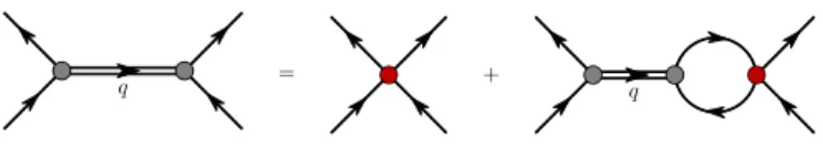
q = +

q

Figure 2. (Colour online) NJL Bethe-Salpeter equation for the quark–antiquarkt-matrix, represented as the double line with the vertices. The single line corresponds to the dressed quark propagator and the BSE ¯qqinteraction kernel, consistent with the gap equation kernel used in Eq. (5), is given by Eq. (2).

duced formally via the relation 1

Xⁿ = 1 (n−1)!

Z ∞ 0

dτ τⁿ⁻¹e^{−τ X},

−→ 1 (n−1)!

Z 1/Λ²_IR

1/Λ²_{U V}

dτ τⁿ⁻¹e^{−τ X}, (6) whereX represents a product of propagators that have been combined using Feynman parametrization. Only the ultraviolet cutoff, ΛU V, is needed to render the the- ory finite, however, for bound states of quarks we also include the infrared cutoff, ΛIR. This has the effect of eliminating unphysical thresholds for the decay of hadrons into free quarks and therefore simulates aspects of quark confinement in QCD.

Mesons in the NJL model are quark–antiquark bound states whose properties are determined by first solving the Bethe-Salpeter equation (BSE). The kernels of the gap and BSEs are intimately related, as exemplified by the vector and axialvector Ward–Takahashi identities, which relate the quark propagator to inhomogeneous Bethe- Salpeter vertices [41]. The NJL BSE, consistent with the gap equation of Fig.1, is illustrated in Fig.2 and reads

T(q) =K+

Z d⁴k

(2π)⁴KS(k+q)S(k)T(q), (7) whereq is the total momentum of the two-body system, T is the two-bodyt-matrix and K is the ¯qq interaction kernel given in Eq. (2). Dirac, colour and isospin indices have been suppressed in Eq. (7). Solutions to the BSE in the ¯qq channels with quantum numbers that correspond to those of the pion,⁵ rho and omega have the form

T^π(q)αβ,γδ= (γ5τi)_αβ τπ(q) (γ5τi)_γδ, (8) T^ρ(q)αβ,γδ= (γµτi)_αβ τ_ρ^µν(q) (γντi)_γδ, (9) T^ω(q)αβ,γδ= (γµ)_αβ τ_ω^µν(q) (γν)_γδ, (10)

5The NJL Lagrangian of Eq. (1) implies that theGρ ψ γ¯ ^µγ5~τ ψ2

¯

qqinteraction should also contribute in the pionic channel, giving rise toπ–a1mixing. However, since thea1meson is much heavier than the pion, the amount of mixing is small and we therefore ignoreπ–a1 mixing in this work.

where τi are the Pauli matrices and τπ(q) = −2i Gπ

1 + 2GπΠP P(q²), (11)

τ_ρ^µν(q) = −2i Gρ

1 + 2GρΠV V(q²)

g^µν+ 2GρΠV V(q²)q^µq^ν q²

, (12) τ_ω^µν(q) = −2i Gω

1 + 2GωΠV V(q²)

g^µν+ 2GωΠV V(q²)q^µq^ν q²

. (13) The functions τπ(q),τ_ρ^µν(q) andτ_ω^µν(q) are the reduced t-matrices, which are interpreted as propagators for the pion, rho and omega mesons. The bubble diagrams in Eqs. (11)–(13) have the form

ΠP P q²

δij= 3i

Z d⁴k

(2π)⁴ Tr [γ5τiS(k)γ5τjS(k+q)], (14) ΠV V(q²)

g^µν−q^µq^ν q²

δij

= 3i

Z d⁴k

(2π)⁴ Tr [γ^µτiS(k)γ^ντjS(k+q)], (15) where the traces are over Dirac and isospin indices. Meson masses are then defined by the pole in the corresponding two-bodyt-matrix.

In a covariant formulation a two-bodyt-matrix, near a bound state pole of massmi, behaves as

T(q)→ Γi(q) Γi(q)

q²−m²_i , (16) where Γi(q) is the normalized homogeneous Bethe- Salpeter vertex function for the bound state. Expanding the t-matrices in Eqs. (8)–(10) about the pole masses gives

Γⁱ_π=p

Zπγ5τi, Γ^µ,i_ρ =p

Zργ^µτi, Γ^µ_ω=p Zωγ^µ,

(17) whereiis an isospin index and the normalization factors are given by

Z_π⁻¹=− ∂

∂q²ΠP P(q²) _q2=m2

π

, (18)

Z_ρ,ω⁻¹ =− ∂

∂q²ΠV V(q²)

q²=m²_ρ,ω. (19) These residues are interpreted as the effective meson- quark-quark coupling constants. Homogeneous Bethe- Salpeter vertex functions are an essential ingredient in, for example, triangle diagrams that determine the meson form factors.

Baryons in the NJL model are naturally described as bound states of three dressed quarks. The properties of these bound states are determined by the relativistic Fad- deev equation whose solution gives the Poincar´e covariant

Faddeev amplitude. To construct the interaction kernel of the Faddeev equation we require the elementary quark- quark interaction kernel. Using Fierz transformations to rewrite Eq. (1) as a sum ofqq interactions, keeping only the isoscalar–scalar (0⁺, T = 0) and isovector–axialvector (1⁺, T = 1) two-body channels, the NJL interaction La-

grangian takes the form L^I,qq=Gs

hψ γ¯ 5C τ2βAψ¯^Tih

ψ^TC⁻¹γ5τ2βAψi +Ga

hψ γ¯ µC τiτ2βAψ¯^Tih

ψ^TC⁻¹γ^µτ2τiβAψi , (20) where C =iγ2γ0 is the charge conjugation matrix and the couplingsGsand Ga give the strength of the scalar and axialvectorqqinteractions. Because only colour ¯3 qq states can couple to a third quark to form a colourless three-quark state, we must have βA = q

3

2λA (A = 2,5,7) [27]. The Lagrangian of Eq. (20) gives the following elementaryqqinteraction kernel

K^αβ,γδ= 4i Gs(γ5C τ2βA)_αβ C⁻¹γ5τ2βA

γδ

+ 4i Ga(γµC τiτ2βA)_αβ C⁻¹γ^µτ2τiβA

γδ. (21) This kernel has been truncated to support only scalar and axialvector diquark correlations because the pseu- doscalar and vector diquark components of the nucleon must predominantly be in`= 1 states and are therefore suppressed. Pseudoscalar and vector diquarks are also usually found to be considerably heavier than their scalar and axialvector counterparts [42].

Using Eq. (21) as the interaction kernel in the Faddeev equation allows us to first sum all two-bodyqqinteractions to form the scalar and axialvector diquark t-matrices.

Diquark correlations in the nucleon are therefore a natural consequence of the strong coupling in the colour ¯3 quark- quark interaction channel. The BSE in theqqchannel for our NJL model reads

T(q) =K+1 2

Z d⁴k

(2π)⁴KS(k+q)S(−k)T(q), (22) whereKis given in Eq. (21) and there is a symmetry factor of ¹₂ relative to the ¯qqBSE of Eq. (7). The solutions to the BSE in the scalar and axialvector diquark channels are

T^s(q)αβ,γδ= (γ5C τ2βA)_αβτs(q) C⁻¹γ5τ2βA

γδ, (23) T^a(q)αβ,γδ= (γµC τiτ2βA)_αβτ_a^µν(q) C⁻¹γντ2τiβA

γδ, (24) where

τs(q) = −4i Gs

1 + 2GsΠP P(q²), (25)

τ_a^µν(q) = −4i Ga

1 + 2GaΠV V(q²)

g^µν+ 2GaΠV V(q²)q^µq^ν q²

. (26)

p

=

p

Figure 3. Homogeneous Faddeev equation for the nucleon in the NJL model. The single line represents the quark propaga- tor and the double line the diquark propagators. Both scalar and axialvector diquarks are included in these calculations.

The scalar and axialvector diquark masses are defined as the poles⁶ in Eqs. (25) and (26), respectively, and the homogeneous Bethe-Salpeter vertices read

Γs=p

Zsγ5C τ2βA, Γ^µ,i_a =p

Zaγ^µC τiτ2βA, (27) whereiis an isospin index. The pole residues are given by

Z_s⁻¹=−1 2

∂

∂q²ΠP P(q²) _q2=M2

s

, (28)

Z_a⁻¹=−1 2

∂

∂q²ΠV V(q²)

q²=M_a², (29) whereMsandMa are the scalar and axialvector diquark masses. These pole residues are interpreted as the effective diquark–quark-quark couplings.

The homogeneous Faddeev equation is illustrated in Fig.3, where diquark correlations have been made explicit.

The relativistic Faddeev equation in the NJL model has been solved numerically in Refs. [47–49], where the in- tegrals were regularized using the Lepage–Brodsky and transverse momentum cutoff schemes. In the proper-time regularization scheme used here, solving the Faddeev equa- tion is much more challenging and we therefore employ the static approximation to the quark exchange kernel.

In this approximation the propagator of the exchanged quark becomes S(k) → −M¹ [47]. The nucleon vertex function then takes the form

ΓN(p) =p

−ZN Γ =p

−ZN

Γs(p) Γ^µ,i_a (p)

=p

−ZN

"

α1

α2 p^µ

MNγ5 +α3γ^µγ5

√τi

3

#

χ(t)u(p), (30)

6 In QCD these poles should not exist, since diquarks, as coloured objects, are not part of the physical spectrum. Nevertheless, diquark states play a very important role in many phenomeno- logical studies, for example in the spin and flavor dependence of nucleon PDFs [43,44]. They have also been observed in lattice QCD studies [45] as well as model studies of QCD, for exam- ple, in the rainbow-ladder truncation of the Dyson-Schwinger equations (DSEs). In the DSE approach diagrams beyond the rainbow-ladder truncation have been shown to remove the pole in the diquarkt-matrix [46].

where i is an isospin index and χN(t) is the nucleon isospinor:

χ ¹₂

= 1

0

, χ −¹2

= 0

1

. (31) The first element in the column vector of Eq. (30) repre- sents the piece of the nucleon vertex function consisting of a quark and scalar diquark, while the second element represents the quark and axialvector diquark component.

The nucleon mass is labelled byMN and the Dirac spinor is normalized such that ¯uNuN = 1. ZN is the nucleon ver- tex function normalization andα1, α2, α3are obtained by solving the Faddeev equation. After projection onto positive parity, spin one-half and isospin one-half, the homogeneous Faddeev equation is given by [27]

ΓN(p, s) =K(p) ΓN(p, s), (32) which in matrix form reads

Γs

Γ^µ_a

= 3 M

ΠN s √

3γαγ5Π^αβ_{N a}

√3γ5γ^µΠN s −γαγ^µΠ^αβ_{N a} Γs

Γa,β

. (33) The quark-diquark bubble diagrams are defined as

ΠN s(p) =

Z d⁴k

(2π)⁴τs(p−k)S(k), (34) Π^µν_{N a}(p) =

Z d⁴k

(2π)⁴τ_a^µν(p−k)S(k). (35) The vertex normalization of Eq. (30) is given by

ZN =

Γ∂ΠN(p)

∂p² Γ −1

p²=M_N²

, (36)

where

ΠN(p) =

ΠN s(p) 0 0 Π^αβ_{N a}(p)

. (37)

Regulating expressions such as those in Eqs. (34) and (35) using the proper-time scheme is tedious. Therefore, to render the Faddeev equation and form factor calculations tractable we make the pole approximation to the meson and diquarkt-matrices, for example, Eqs. (25) and (26) become

τs(q)→ − i Zs

q²−M_s²+i ε, (38) τ_a^µν(q)→ − i Za

q²−M_a²+i ε

g^µν−q^µq^ν M_a²

. (39) Similar expressions are obtained in the meson sector.

In summary, the model parameters consist of the two regularization scales ΛIR and ΛU V, the dressed quark massM,⁷and the Lagrangian coupling constantsGπ,Gρ,

7Alternatively, one could specify a current quark mass, as one determines the other through the gap equation.

ΛIR ΛU V M Gπ Gρ Gω Gs Ga

0.240 0.645 0.4 19.0 11.0 10.4 5.8 4.9 Table I. Model parameters constrained to reproduce the physi- cal pion, rho and omega masses; the pion decay constant; and the nucleon and delta baryon masses. The infrared regulator and the dressed quark mass are assigned their valuesa priori.

The regularization parameters and dressed quark mass are in units of GeV, while the couplings are in units of GeV⁻².

Gω, Gs, Ga. The infrared regularization scale is associ- ated with confinement and therefore should be of the order ΛQCD, and we choose ΛIR= 0.240 GeV and for the con- stituent quark mass takeM = 0.4 GeV. The physical pion mass (mπ = 140 MeV) and decay constant (fπ= 92 MeV) determine ΛU V andGπ. The physical masses of the rho (mρ = 770 MeV) and omega (mω = 782 MeV) mesons constrainGρ andGω, respectively, while the physical nu- cleon (MN = 940 MeV) and ∆ (M∆= 1232 MeV) baryon masses determineGsandGa.⁸ Numerical values are given in Tab.I.

Using the parameters given in Tab.I, we obtain the fol- lowing results for the residues of the two-bodyt-matrices:

Zπ = 17.9, Zρ = 6.96, Zω = 6.63, Zs = 11.1 and Za = 6.73. For the nucleon vertex function of Eq. (30) we find ZN = 28.1 and (α1, α2, α3) = (0.55,0.05,−0.40), where the scalar and axialvector diquark masses are Ms= 0.768 GeV andMa = 0.903 GeV.

III. NUCLEON ELECTROMAGNETIC CURRENT

The electromagnetic current of an on-shell nucleon, expressed in terms of the Dirac and Pauli form factors, has the form

j_λ^µ0λ(p⁰, p) =hp⁰, λ⁰|J_em^µ |p, λi

=u(p⁰, λ⁰)

γ^µF1(Q²) +iσ^µνqν

2MN

F2(Q²)

u(p, λ), (40) where q=p⁰−pis the 4-momentum transfer,Q²≡ −q² andλ,λ⁰ represent the initial and final nucleon helicity respectively. The nucleon’s electric and magnetic Sachs form factors [50], which diagonalize the Rosenbluth cross- section, are then given by

GE(Q²) =F1(Q²)− Q²

4M_N² F2(Q²), (41) GM(Q²) =F1(Q²) +F2(Q²). (42) Hadron form factors can be decomposed into a sum over the quark charges multiplied by quark sector form

8 The relativistic Faddeev equation for the Delta baryon is discussed, for example, in Ref. [27].

factors, such that

Fh(Q²) = X

q eqF_h^q(Q²). (43) The quark sector form factorsF_h^q(Q²) represent the con- tribution of the current quarks of flavourq to the total hadron form factorFh(Q²). The proton and neutron form factors expressed in terms of quark sector form factors read

Fip(Q²) =euF_ip^u(Q²) +edF_ip^d(Q²) +. . . (44) Fin(Q²) =euF_in^u(Q²) +edF_in^d(Q²) +. . . (45) where i = 1,2. Note that in light of the experimental discovery that the strange quarks contribute very little to the nucleon electromagnetic form factors [51–54], we will neglect their contribution to Eqs. (44) and (45). Assum- ing equaluanddcurrent quark masses and neglecting electroweak corrections, theu anddquark sector form factors of the nucleon must satisfy the charge symmetry constraints:

F_in^d(Q²) =F_ip^u(Q²) and F_in^u(Q²) =F_ip^d(Q²). (46) Experimentally, if electroweak and heavy quark effects are small, theuanddquark sector form factors are given accurately by

F_ip^u = 2Fip+Fin, F_ip^d =Fip+ 2Fin. (47) Recent accurate data for the neutron form factors has enabled a precise determination of the quark sector proton form factors [55]. We will discuss results for these quark sector form factors in Sect.VI.

The slope of an electromagnetic form factor at Q²= 0 is a measure of either the squared rms charge or magnetic radius of a hadron. Unless stated otherwise all squared rms radii are defined by

r²

=−6 η

∂ f(Q²)

∂Q² _Q2=0

η=

(1 iff(0) = 0, f(0) iff(0)6= 0, (48) wheref(Q²) is an arbitrary form factor. This definition reproduces the standard nucleon results for the charge and magnetic radii defined by the Sachs form factors:

r²_E

=−6 ∂ GE(Q²)

∂Q²

_Q2=0, (49) r²_M

=− 6

GM(0)

∂ GM(Q²)

∂Q²

_Q2=0, (50) but also generalizes to radii defined with respect to the Dirac and Pauli form factors and quark sector form factors.

Hadronic radii, in units of fm, will be obtained from the result of Eq. (48) using

r≡sign r² p

|hr²i|. (51)

p p^′ q

+

p q p^′

Figure 4. (Colour online) Feynman diagrams representing the nucleon electromagnetic current. The diagram on the left is called thequark diagram and the diagram on the right the diquark diagram. In the diquark diagram the photon interacts with each quark inside the non-pointlike diquark.

To calculate the nucleon electromagnetic current and therefore the Dirac and Pauli form factors, one must know the manner in which the nucleon described in Sect.IIcou- ples to the photon, guaranteeing electromagnetic gauge invariance. The necessary Feynman diagrams are illus- trated in Fig.4and a proof of gauge invariance is given in App.B. We include both scalar and axialvector diquarks in our nucleon wave function and therefore the diagrams in Fig.4represent six distinct Feynman diagrams. The diagram on the left, referred to as the quark diagram, represents the processes where the photon couples to a dressed quark with either a scalar or axialvector diquark as a spectator. Thediquark diagram, on the right in Fig.4, represents four Feynman diagrams; the photon can couple to a scalar diquark, an axialvector diquark or cause a transition between these two diquark states. Importantly, in thediquark diagram the photon couples to the quarks inside each diquark, thereby resolving internal diquark structure and resulting in, for example, diquarks with a finite size. The coupling of a photon to a dressed quark and to the diquarks is discussed in Sects.IVandV.

IV. QUARK–PHOTON VERTEX

The quark-photon vertex in the NJL model, and other field theoretic approaches, is given by the solution to an inhomogeneous BSE. The NJL model version of this equa- tion, consistent with the truncation used in the gap and BSEs discussed Sect.II, is represented diagrammatically in Fig.5. The large oval represents the quark-photon ver- tex, Λ^µ_γQ(p⁰, p), the 4-fermion interaction kernel is given in Eq. (2) and the elementary vertex, which gives the inhomogeneous driving term, has the formγ^µQˆ (where Qˆ is the quark charge operator). The second equality in Fig.5expresses this equation in an equivalent form using the ¯qq t-matrices.

The quark charge operator is Qˆ =

eu 0 0 ed

=1 6 +τ3

2, (52)

whereeu= ²₃ anded=−¹3 are theuanddquark charges.

The quark-photon vertex therefore has both an isoscalar and isovector component, which may in general be ex-

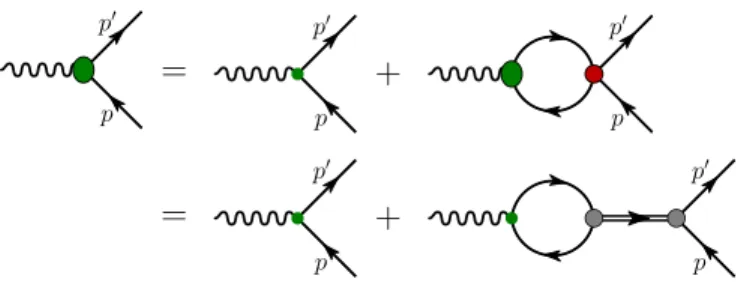
p p^′

=

p p^′

+

p p^′

=

p p^′

+

p p^′

Figure 5. (Colour online) Inhomogeneous Bethe-Salpeter equa- tion whose solution gives the quark-photon vertex, represented as the large shaded oval. The small dot is the inhomogeneous driving term, while the shaded circle is the ¯qq interaction kernel given in Eq. (2). Only theρandωinteraction channels contribute. This integral equation can equivalently be repre- sented using the elementary quark-photon interaction and the ρandω t-matrices, given in Eqs. (12) and (13). This case is depicted by the second equality.

pressed in the form

Λ^µ_γQ(p⁰, p) = 1

6Λ^µ_ω(p⁰, p) +τ3

2 Λ^µ_ρ(p⁰, p). (53) The quark-photon vertex, separated into flavour sectors defined by the dressed quarks, reads

Λ^µ_γQ(p⁰, p) = Λ^µ_U(p⁰, p) 1 +τ3

2 + Λ^µ_D(p⁰, p) 1−τ3

2 . (54) In general each dressed quark component of the quark- photon vertex contains contributions from both the u anddcurrent quarks. This will prove important when we consider quark sector form factors and associated charge symmetry constraints. Note that throughout this manuscript we use a capitalQ= (U, D) to indicate that an object is associated with dressed quarks and a lowercase q= (u, d) to represent the current quarks of the NJL and QCD Lagrangians.

The quark-photon vertex has in general 12 Lorentz structures [56], 4 longitudinal and 8 pieces transverse to the photon momentum, where each Lorentz structure is accompanied by a scalar function of the three variables q², p⁰²andp².⁹ The standard NJL ¯qqinteraction kernel, as employed in Sect.II for the gap and BSE equations, is momentum independent which implies that the quark- photon vertex can only depend on the momentum transfer q =p⁰−p, not p⁰ and pseparately. Therefore, in this work, the contributions to the vertex functions of Eq. (53)

9The 12 Lorentz structures in the quark-photon vertex are not all independent, since, for example, the Ward–Takahashi identity and time reversal invariance place additional constraints.

from the NJL BSE, take the form Λ^(bse)µ_ω (q) =γ^µ+

γ^µ−q^µ/q q²

Fˆ1ω(q²) +iσ^µνqν

2M F2ω(q²), (55) Λ^(bse)µ_ρ (q) =γ^µ+

γ^µ−q^µ/q q²

Fˆ1ρ(q²) +iσ^µνqν

2M F2ρ(q²).

(56) With the quark propagator of Eq. (4), these results satisfy the Ward–Takahashi identity:

qµΛ^µ_γQ(p⁰, p) = ˆQ

S⁻¹(p⁰)−S⁻¹(p)

, (57) demanded byU(1) vector gauge invariance.

Current conservation at the hadron level implies that theq^µ/q/q² term in Eqs. (55) and (56) cannot contribute to hadron form factors. We therefore write our effective vertex as

Λ^(bse)µ_i (q) =γ^µF1i(q²) +iσ^µνqν

2M F2i(q²), (58) where i = (ω, ρ) and F1i(q²) = 1 + ˆF1i(q²). This ver- tex has the same form as the electromagnetic current for an on-shell spin-half fermion. For a pointlike quark F1ω(q²) = 1 =F1ρ(q²) andF2ω(q²) = 0 =F2ρ(q²). How- ever, interactions in the NJL model not only dynamically generate a dressed quark mass but also generate non- trivial dressed quark form factors.

The inhomogeneous BSE for the quark-photon vertex, depicted in Fig.5, has the form

Λ^µ_γQ(p⁰, p) =γ^µ 1

6 +τ3

2

+X

ΩKΩΩ

× i Z d⁴k

(2π)⁴ Trh

Ω¯S(k+q) Λ^µ_γQ(p⁰, p)S(k)i , (59) where P

ΩKΩ ΩαβΩ¯λε represents the interaction ker- nel given in Eq. (2). The Dirac and isospin structure of Λ^µ_γQ(p⁰, p), given in Eqs. (53), (55) and (56), im- plies that of the interaction channels in Eq. (2) only the isovector–vector,−2i Gρ(γµ~τ)_αβ(γ^µ~τ)_γδ, and isoscalar–

vector,−2i Gω(γµ)_αβ(γ^µ)_γδ, pieces can contribute.

The dressed quark form factors obtained from the in- homogeneous BSE, associated with the electromagnetic current of Eq. (58), are

F1i(q²) = 1

1 + 2GiΠV V(q²), F2i(q²) = 0, (60) where i = ω, ρ. Comparison with Eqs. (12) and (13) indicate thatF1ω andF1ρ have a pole at q² =m²_ω and m²_ρ, respectively. The NJL BSE kernel of Eq. (2) does not generate Pauli form factors for the dressed quarks because it does not include the tensor–tensor 4-fermion interaction. The dressed up and down quark form factors given by the BSE therefore read

F_1Q^(bse)(Q²) = 1

6F1ω(Q²)±1

2F1ρ(Q²), (61)

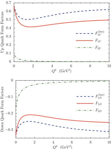
0 0.1 0.2 0.3 0.4 0.5 0.6 0.7

UpQuarkFormFactors

0 2 4 6 8 10

Q² (GeV²)

F_1U^(bse) F1U

F2U

−0.3

−0.2

−0.1 0

DownQuarkFormFactors

0 2 4 6 8 10

Q² (GeV²)

F_1D^(bse) F1D

F2D

Figure 6. (Colour online)Upper panel: Dressed up quark form factors: the dashed line is the Dirac form factor obtained from the BSE of Eq. (59); the solid and dash-dotted lines are respectively the Dirac and Pauli form factors generated by also including the pion loop corrections illustrated in Fig.8.

Lower panel: Dressed down quark form factors: each curve represents an analogous form factor to those in the upper panel.

where the plus sign is associated with a dressed up quark.

The superscript (bse) indicates that these form factors are obtained solely from the BSE.

Results for the dressed quark BSE form factors are illustrated as the dashed lines in Figs. 6. A notable feature of these results is that they do not drop to zero asQ²→ ∞, but instead behave as

F_1U^(bse)(Q²)^Q

2→∞

= eu, F_1D^(bse)(Q²)^Q

2→∞

= ed, (62) signifying that at infiniteQ² the photon interacts with a bare current quark. This result is consistent with QCD expectations based on asymptotic freedom.

Pion loop corrections to the quark-photon vertex will also be considered and treated as a perturbation to the dressed quark form factors obtained from the BSE, as given in Eqs. (60) and (61). In this case the dressed quark propagator receives an additional self-energy correction

p k p p−k

β α

j i

Figure 7. (Colour online) Pion loop contribution to the dressed quark self-energy. The pion couples to the dressed quark via γ5τiand the piont-matrix is approximated by its pole form.

which is illustrated in Fig.7.¹⁰ In addition to the pionic self-energies on the dressed quarks, pion exchange between quarks should also be included in the two-body kernels that enter the Bethe-Salpeter and Faddeev equations.

However, it is straightforward to show that in the limit where the nucleon and ∆ are mass degenerate, including only self-energy correction on the dressed quarks yields essentially the correct leading non-analytic behaviour of the electromagnetic form factors as a function of quark mass. Further, in form factor calculations diagrams with a photon coupling to an exchanged pion do not contribute because of the cancellation betweenπ⁺andπ⁻ exchange.

This self-energy is evaluated using a pole approximation, where the external quark is assumed on-mass-shell. The pion loop therefore shifts the dressed quark mass by a constant, giving a quark propagator of the form

S(k) =˜ Z S(k), Z= 1 + ∂Σ(p)

∂/p /p=M

, (63) whereS(k) is the usual Feynman propagator for a dressed quark of mass¹¹ M and the self-energy reads¹²

Σ(p) =− Z d⁴k

(2π)² γ5τiS(p−k)γ5τiτπ(k). (64) When evaluating Σ(p) the reduced pion t-matrix is ap- proximated by its pole form, that is

τπ(k)→ i Zπ

k²−m²_π+iε. (65) The quark wave function renormalization factor, Z, rep- resents the probability to strike a dressed quark without

10Chiral symmetry as expressed in the the NJL Lagrangian of Eq. (1) demands that the sigma meson be included also, however since the sigma has charge zero and (in this work)mπ/mσ'0.18, these additional correction are small and will not be included.

11When including pion loops on the dressed quarks we renormalize theGπcoupling in the NJL Lagrangian to keep the dressed quark mass fixed.

12The pion–quark-quark vertex in Fig.7can be read directly from the piont-matrix, given by Eq. (8), and takes the formγ5τi. A pseudovector component to the vertex would be generated throughπ–a1 mixing in the BSE kernel, however the strength of this vertex is suppressed bymπ/ma₁ ∼0.1 relative to the dominant pseudoscalar component. Therefore, we do not include aπ–a1 mixing in the pion–quark-quark vertex.

p p^′

µ

q

Z× +

p p^′

µ

q k

+ p k p^′

µ

q

Figure 8. (Colour online) Pion loop contributions to the quark- photon vertex. The quark wave function renormalization factor Zrepresents the probability of striking a dressed quark without a pion cloud. In the first two diagrams the photon couples to the dressed quark with a vertex of the general form given by Eq. (53); and defined by Eqs. (58) and (60). The shaded oval in the third diagram represents the quark–pion vertex, which we approximate by its pole form. It is therefore given by (`<sup>0</sup>+`)Fπ(Q²), whereFπ(Q²) is the usual pion form factor (see Eq. (86) and associated discussion).

the pion cloud and is essential to maintain charge conser- vation. Using the parameters in Tab.Igives Z = 0.80.

The quark electromagnetic current, including pion loops, is illustrated in Fig.8. Evaluating this current between on-shell constituent quarks, gives for the dressed quark sector currents of Eq. (54):

Λ^µ_Q(p⁰, p) =γ^µF1Q(Q²) +iσ^µνqν

2M F2Q(Q²), (66) whereQ= (U, D). The dressed quark form factors read

F1U =Z₁

6F1ω+¹₂F1ρ

+ [F1ω−F1ρ]f₁^(q)+F1ρf₁^(π), (67) F1D=Z₁

6F1ω−¹2F1ρ

+ [F1ω+F1ρ]f₁^(q)−F1ρf₁^(π), (68) F2U = [F1ω−F1ρ]f₂^(q)+F1ρf₂^(π), (69) F2D= [F1ω+F1ρ]f₂^(q)−F1ρf₂^(π), (70) where theQ² dependence of each form factor has been omitted. The body form factors,f₁^(q)andf₂^(q), originate from the second diagram in Fig.8, whilef₁^(π) andf₂^(π) are the body form factors from the third diagram, which also contain the pion body form factor (see discussion associated with Eq. (86)). These body form factors are illustrated in Fig. 9. When evaluating the pion loop diagrams in Figs.7and8we use the proper-time regu- larization scheme, however, in this case the pions should not be confined and we therefore set ΛIR= 0 GeV. This procedure guarantees that the leading-order non-analytic behaviour of the hadron form factors as a function of the pion mass is retained.

Results for the Dirac and Pauli dressed quark form factors, including pion loop effects, are given in Figs.6.

The pion cloud softens the Dirac form factors, however its most important consequence is the non-zero Pauli form factor for the dressed quarks. At infiniteQ² the dressed quark Dirac form factors now become

F1U(Q²)^Q

2→∞

= Z eu, F1D(Q²)^Q

2→∞

= Z ed, (71)

−0.05 0 0.05 0.10 0.15

QuarkBodyFormFactors

0 2 4 6 8 10

Q² (GeV²) f₁^(q) f₁^(π)

f₂^(q) f₂^(π)

Figure 9. (Colour online) Dressed quark body form factors associated with the pion loop corrections, wheref₁^(q)andf₂^(q) originate from the second diagram in Fig.8andf₁^(π)andf₂^(π) from the third diagram.

whereas the Pauli form factors vanish for large Q². We find dressed quark anomalous magnetic moments of

κU = 0.10 and κD=−0.17, (72) defined asκQ ≡F2Q(0). The quark charge and magnetic radii, defined with respect to the Sachs form factors and Eq. (48), take the values

r^U_E= 0.59 fm, r_M^U = 0.60 fm, (73) r^D_E = 0.73 fm, r_M^D = 0.67 fm. (74) Decomposing the dressed quark form factors in quark/flavour sectors gives

F1U(Q²) =euF_1U^u (Q²) +edF_1U^d (Q²), (75) F1D(Q²) =euF_1D^u (Q²) +edF_1D^d (Q²), (76) where the flavour sector dressed up quark form factors read

F_1U^u =Z¹₂[F1ω+F1ρ] + [3F1ω−F1ρ]f₁^(q)+F1ρf₁^(π), (77) F_1U^d =Z¹₂[F1ω−F1ρ] + [3F1ω+F1ρ]f₁^(q)−F1ρf₁^(π),

(78) F_2U^u = [3F1ω−F1ρ]f₂^(q)+F1ρf₂^(π), (79) F_2U^d = [3F1ω+F1ρ]f₂^(q)−F1ρf₂^(π). (80) The flavour sector dressed down quark form factors are given by

F_iD^u =F_iU^d and F_iD^d =F_iU^u (81) where i= (1,2). Therefore, these results satisfy charge symmetry and are illustrated in Figs.10. For the quark sector anomalous magnetic moments we find

κ^u_U = 0.02 and κ^d_U =−0.25, (82) and therefore thedcurrent quarks carry the bulk of the dressed up quark anomalous magnetic moment. This will have important implications for the nucleon form factors.

0 0.2 0.4 0.6 0.8 1.0

Fq 1Uquarksectorformfactors

0 1 2 3 4 5

Q² (GeV²)

F_1U^u

F_1U^d

−0.25

−0.20

−0.15

−0.10

−0.05 0

Fq 2Uquarksectorformfactors

0 1 2 3 4 5

Q² (GeV²)

F_2U^u

F_2U^d

Figure 10. (Colour online)Upper panel: Dressed up quark Dirac form factors, that also include pion cloud effects, sepa- rated into quark sectors. The solid line is theu-quark sector of the dressed up quark and the dashed line representsd-quark sector. Lower panel: Dressed up quark Pauli form factors separated into quark sectors. The solid line is theu-quark sector and the dashed line thed-quark sector.

V. DIQUARK AND MESON FORM FACTORS Critical to our picture of nucleon structure are diquark correlations inside the nucleon. An essential step there- fore, in calculating the nucleon form factors, is to first determine the interaction of the virtual photon with the diquarks. A further reason to discuss the diquark form factors is that the scalar and axialvector diquarks are the qqanalogs of theπandρmesons.

The electromagnetic current of a diquark is represented by the Feynman diagrams illustrated in Fig.11 and is expressed as

j^µ(p⁰, p) =i Z d⁴k

(2π)⁴ Trh

Γ(p⁰)S(p⁰+k) Λ^µ_γQ(p⁰, p)S(p+k) Γ(p)S^T(−k)i , (83) where the superscriptT indicates transpose. The Bethe- Salpeter vertices are represented by Γ(p) and are given