Spread of Chaotic Behavior
in Switching Ring Network Topology by Coupled Chaotic Circuits
Takahiro Chikazawa, Yoko Uwate and Yoshifumi Nishio Dept. of Electrical and Electronic Engineering, Tokushima University
2-1 Minami-Josanjima, Tokushima 770–8506, Japan Email:{chikazawa,uwate,nishio}@ee.tokushima-u.ac.jp
Abstract—In this study, we investigate the spread of chaotic behavior in switching ring network topology. We propose ring network model by coupled chaotic circuits. In proposed network model, one circuit is set to generate chaotic attractor and the other circuits are set to generate three-periodic attractors. By using computer simulations, we investigate the chaos propagation by changing the switching coupling patterns. From the simulation result, the chaos propagation depends on the previous switching pattern.
I. INTRODUCTION
We have various types network in our society. Most of networks can be represented as a graph by nodes and edges.
Moreover, the network model has various types of feature quantities. Examples of feature quantities are path length, de- gree distribution and clustering coefficient. However, network model become more large scale and complicated network.
These network model is called by complex networks . Recently, complex networks have attracted a great deal of attention from various fields since the discovery of small- world network [1] and scale-free network [2]. As with the complex networks, various types of propagation in complex network have attracted a great deal of attention from various fields. For example, friendship in social network, neural activities with information processing in human brain network and the pandemic outbreak of viral infection in biology. Therefore, we consider that we can analyze various complicated phenomena of complex networks by investigating the spread of chaotic behavior. Additionally, it is important to investigate propagation phenomena observed from coupled chaotic circuits for future engineering applications.
In our research group, we have investigated the spread of chaotic behavior in various type networks. Various research results of spread of chaotic behavior in static network model have been reported by using coupled chaotic circuits [3]. In this study, we confirmed that the three-periodic attractors are affected from the chaotic attractors when the coupling strength increases. In scale free network, we confirmed that chaos propagation is more difficult when we set the initial chaos position in high degree node. Additionally, we have compared scale free and random network for investigation spread of
chaotic behavior [4]. Even though we increase the value of degree in initial chaos position, the ratio of propagation changes only a little. In detail of this result, we explain this result in section(III).
However, these previous study have been reported by static network model. Therefore it is necessary to investigate the spread of chaotic behavior in dynamic network model. Ex- ample of dynamic network model is temporal networks [5].
Figure 1 shows the example of temporal networks. In addition, various research of propagation by using temporal networks have been reported by many researchers [6].
Fig. 1. System model of temporal networks.
In this study, we propose ring network model by 10 coupled chaotic circuits. In ring network of initial state, we fixed that one circuit is set to generate chaotic attractor and the other cir- cuits are set to generate three-periodic attractors. Additionally, we switch the network topology such as temporal networks.
We propose two different switching coupling patterns. We define these patterns that we cut two edges at every switching time. In these conditions, we investigate the spread of chaotic behavior in switching ring network topology.
II. CIRCUIT MODEL
The chaotic circuit is shown in Fig. 2. This circuit consists of a negative resistor, two inductors, a capacitor and dual- directional diodes. This chaotic circuit is called Nishio-Inaba circuit.
The circuit equations of this circuit are described as follows:
- 111 -
IEEE Workshop on Nonlinear Circuit Networks December 15-16, 2017
i
1i
2L
1-r C v
v
dL
2C n
Fig. 2. Chaotic circuit.
L1
di
dt =v+ri L2
di
dt =v−vd
Cdv
dt =−i1−i2,
(1)
The characteristic of nonlinear resistance is described as follows:
vd= rd
2
(i2+ V rd
− i2− V
rd )
. (2)
By changing the variables and parameters,
i1=
√C L1
V xn, i2=
√L1C L2
V yn, v=V zn
α=r
√C L1
, β= L1
L2
, δ=rd
√L1C L2
,
γ= 1 R
√L1
C , t=√ L1C2τ,
(3)
The normalized circuit equations are given as follows:
dxi
dτ =αxi+zi
dyi
dτ =zi−f(yi) dzi
dτ =−xi−βyi− ∑
j∈Sn
γ(zi−zj) (i, j = 1,2,· · ·, N).
(4)
In Eq. (4),N is the number of coupled chaotic circuits and γ is the coupling strength.f(yi)is described as follows:
f(yi) =1 2
(yi+ 1 δ
− yi− 1
δ )
. (5)
In Eq. (4), N is the number of coupled chaotic circuits and γ is the coupling strength. We defineαc to generate the chaotic attractor (see Fig. 3(a)) andαp is defined to generate the three-periodic attractors (see Fig. 3(a)). For the computer simulations, we calculate Eq. (4) using the fourth-order Runge- Kutta method with the step size h = 0.01. In this study, we set the parameters of the system as αc= 0.460,αp= 0.418, β= 3.0andδ= 470.0.
z
x
(a)Chaotic attractor (b)Three-periodic attractor
x
z
Fig. 3. Attractor.
III. STATIC NETWORK MODEL IN PREVIOUS STUDY[4]
In this section, we investigate the ratio of propagation in static complex model.
A. System model
Figures 3 and 4 show the proposed different type network models in our previous study [6]. The characteristic of Model- A is the scale-free network topology. The characteristic of Model-B is the random network topology. In each model, each chaotic circuit is coupled by one resistor R. We use 25 coupled chaotic circuits and 34 resistors in each network model. Moreover, these proposed network model is static network model.
Figure 5 shows degree distribution of each network. In this graph, the vertical axis denotes the number of nodes and the horizontal axis denotes the value of degree.
1 2
3 4 5 6
8 7 9 10
11
12 13
14 15
16 17
18
19
20 21
22 23
24 25
Fig. 4. Model-A (Scale-free network).
4 5
19 25 24
11 23
1 2
3 10
6 13
14 15
12 20 7 8 9
16
18 21 17
22
Fig. 5. Model-B (Random network).
Fig. 6. Degree distribution of each network..
- 112 -
B. Simulation result
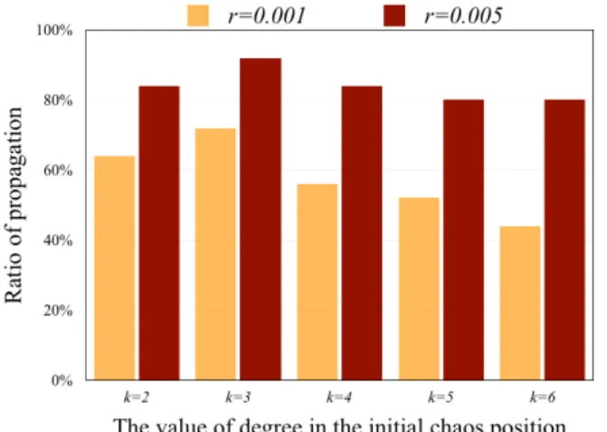
We investigate the ratio of propagation when we change the value of degree in the initial chaos position according to degree distribution. Moreover, in scale-free and random networks, we compare their differences of simulation results. For example, in model-A, when the value of degree k in the initial chaos position is 4, we set the chaotic attractor in 9th or 13th node.
Also, in model-B, when the value of degree k in the initial chaos position is 4, we set the chaotic attractor in 9th or 17th node.
The simulation results of ratio of propagation according to degree distribution are shown in Figs. 6 and 7.
Furthermore, we average the ratio of propagation in each node under the same condition. In addition, we investigate the ratio of propagation in the static state when we fix coupling strength as γ = 0.001,0.005. Here, we define the ratio of propagation as number of chaotic circuits of whole network at steady state.
Fig. 7. Ratio of propagation according to degree distribution in Model- A (scale-free network).
Fig. 8. Ratio of propagation according to degree distribution in Model- B (Random network).
From the result, in scale-free network, chaos propagation become to more difficult, when we increase the value of degree in initial chaos position. On the other hand, in random network, even though we increase the value of degree in initial chaos position, the ratio of propagation changes only a little.
IV. DYNAMIC NETWORK MODEL
In this section, we investigate the spread of chaotic behavior in dynamic model.
A. Switching coupling pattern
Figure 9 shows the proposed ring network model in this study. In the proposed model, each chaotic circuit is coupled by one resistorR. We use 10 coupled chaotic circuits and 10 edges.
1st 2nd
3rd
4th
5th
6th
7th
8th 9th 10th
R
Fig. 9. Ring network model.
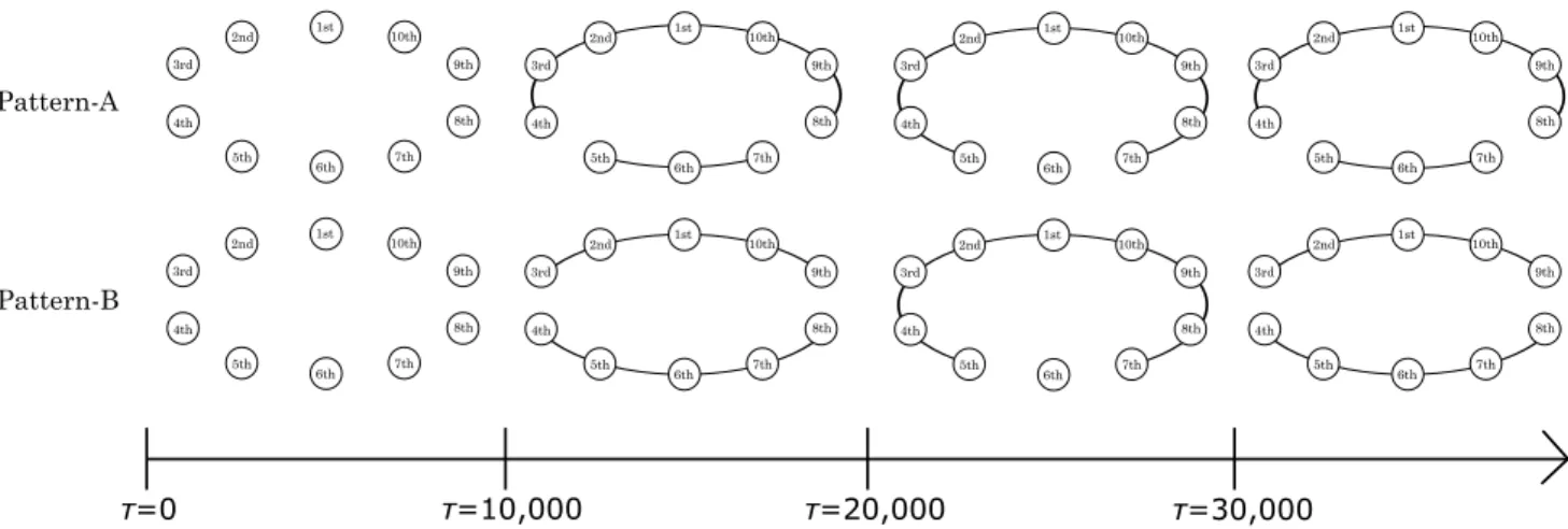
We propose two different switching coupling patterns in Fig. 10. In this study, we change the switching coupling patterns at every τ = 10,000. Moreover, in every switching, we cut the two edges.
In pattern-A, all edges are cut form τ = 0toτ = 10,000.
Next switching, we cut two edges from 4th to 5th node and from 7th to 8th node. Next switching, we cut two edges from 5th to 6th node and from 6th to 7th node. Finally, we cut two edges from 4th to 5th node and from 7th to 8th node.
In pattern-B, all edges are cut form τ = 0 toτ = 10,000.
Next switching, we cut two edges from 3rd to 4th node and from 8th to 9th node. Next switching, we cut two edges from 5th to 6th node and from 6th to 7th node. Finally, we cut two edges from 3rd to 4th node and from 8th to 9th node.
B. Simulation results
We investigate the chaos propagation by changing the switching coupling patterns. In the initial states of each pattern, one circuit is set to generate chaotic attractor and the other circuits are set to generate three-periodic attractors. We set the initial chaos position in 6th node and the other node is fixed as three-periodic state. In addition, we investigate the chaos propagation in the static state when we fix coupling strength asγ= 0.010. Figure 11 shows the appearances how to spread from three-periodic state to chaotic state when we change the switching coupling according to pattern-A. Moreover, Fig. 12 shows the appearances how to spread from three-periodic attractor to chaotic attractor when we change the switching coupling according to pattern-B.
- 113 -
1st 2nd 3rd
4th
5th 6th
7th 8th 9th 10th
1st 2nd 3rd
4th
5th 6th
7th 8th 9th 10th
1st 2nd 3rd
4th
5th 6th
7th 8th 9th 10th
τ=0 τ=10,000 τ=20,000 τ=30,000
1st 2nd 3rd
4th
5th 6th
7th 8th 9th 10th 1st
2nd 3rd
4th
5th 6th
7th 8th 9th
10th 1st
2nd 3rd
4th
5th 6th
7th 8th 9th 10th 1st
2nd 3rd
4th
5th 6th
7th 8th 9th 10th 1st
2nd 3rd
4th
5th 6th
7th 8th 9th 10th
Pattern-A
Pattern-B
Fig. 10. Switching coupling pattern at everyτ= 10,000.
1st 2nd 3rd 4th 5th 6th 7th 8th 9th 10th
τ=0
τ=10,000
τ=20,000
τ=30,000
Fig. 11. spread of chaotic behavior in pattern-A.
1st 2nd 3rd 4th 5th 6th 7th 8th 9th 10th
τ=0
τ=10,000
τ=20,000
τ=30,000
Fig. 12. spread of chaotic behavior in pattern-B.
From each simulation result, we have observed the chaos propagation. In switching time from τ = 10,000 to τ = 20,000, in each switching pattern, each three-periodic at- tractors which is connected to 6th node are changed to chaotic state by the influence of 6th node. In pattern-A from τ = 20,000 to τ = 30,000, 5ht and 7th node change to three-periodic state because the edges from 5th to 6th node and from 6th to 7th node are cut. However, in pattern-B from τ = 20,000 to τ = 30,000, despite the fact that the both side edges of 6th node do not connect to other nodes, we observed that three-periodic state node change to chaotic state.
Moreover, in switching time from τ = 30,000toτ = 40,000 of pattern-B, only 4th, 5ht, 7th and 8th node keep at chaotic state because the both side edges of 5ht, 6th and 7th node are connected.
V. CONCLUSIONS
In this study, we have investigated the spread of chaotic behavior in switching ring network topology by coupled chaotic circuits. By the computer simulations, we confirmed that the three-periodic state is affected from the chaotic state.
Moreover, we have observed the spread of chaotic behavior by the influence of switching pattern. From the simulation result, we consider that the spread of chaotic behavior depends on previous switching coupling pattern. Even if the edge temporarily connect to other nodes, it is assumed that we observe the chaos propagation by changing the switching coupling pattern.
For the future works, we propose the different switching pattern such as random or systematic. Furthermore, we in- vestigate the spread of chaotic behavior when we change the switching coupling patterns at every more shortτ.
REFERENCES
[1] D. J. Watts and S. H. Strogatz, “Collective dynamics of small-world , Nature, vol. 393, pp. 440-442, 1998.
[2] A. L. Barabasi and R. Albert, Emergence of scaling in random networks , Science, vol. 286, pp. 509-512, 1999.
[3] T. Chikazawa, Y. Uwate and Y. Nishio, “Investigation of Spreading Chaotic Behavior in Coupled Chaotic Circuit Networks with Various Features,” Proceedings of RISP International Workshop on Nonlinear Circuits, Communications and Signal Processing (NCSP’17), pp. 337- 340, Feb. 2017.
[4] T. Chikazawa, Y. Uwate and Y. Nishio, “Spread of Chaotic Behavior in Scale-Free and Random Networks,” Proceedings of Asia Pacific Con- ference on Postgraduate Research in Microelectronics and Electronics (PrimeAsia’17), pp. 21-24, Oct. 2017.
[5] P. Holme, J Saramaki, “Temporal networks,” Physics Reports, vol. 519, Issue 3, pp. 97-125, Oct 2012.
[6] B. Adhikari, Y. Zhang, A. Bharadwaj, B. A. Prakash,“Condensing Temporal Networks using Propagation,” Proceedings of the 2017 SIAM International Conference on Data Mining, pp. 417-425, Apr 2017.
![Figure 1 shows the example of temporal networks. In addition, various research of propagation by using temporal networks have been reported by many researchers [6].](https://thumb-ap.123doks.com/thumbv2/123deta/7315782.2423500/1.892.455.813.601.712/temporal-networks-addition-research-propagation-temporal-networks-researchers.webp)