2 Parallel Simulated Annealing

(1)

Parallel Simulated Annealing using Genetic Crossover

Tomoyuki HIROYASU^†, Mitsunori MIKI^†, and Maki OGURA^††

† Department of Knowledge Engineering,

†† Graduate School of Engineering, Doshisha University

Kyo-tanabe, Kyoto, 610-0321, JAPAN Email: [email protected]

Abstract

This paper proposes a new algorithm of a simulated annealing(SA): Parallel Simulated Annealingusing Genetic Crossover (PSA/GAc). The proposed algorithm consists of several processes, and in each process SA is operated. The genetic crossover is used to exchange information between solutions at ﬁxed in- tervals. While SA requires high computational costs, particularly in continuous problems, this operation reduces the computational cost. The proposed algorithm is applied to continuous test problems. It is found that the proposed algorithm can search the global optimum solution eﬀectively, compared to distributed genetic algorithms and sequential simulated annealing.

keywords: Optimization Problems, Parallel Dis- tributed Algorithms, Simulated Annealing, Ge- netic Crossover, Hybrid Algorithm

1 Introduction

Simulated Annealing(SA) is one of the emergent cal- culation algorithms that solves optimization problems, and is an eﬀective technique for solvingcombination optimization problems[1]. SA is an algorithm that sim- ulates the physical evolution of a solid from a high temperature state to a thermal equilibrium state[2].

SA searches randomly around the neighborhood of a present searchingpoint. The next searchingpoint can be accepted even when the fitness value of the next point is worse than that of the present. SA algorithms repeat these steps, and the optimization state is finally expected from given initial state[1][3]. Therefore, it can derive the global solution. However, SAs require huge computational cost. Specifically, SA takes much time findingthe optimum solution in continuous problems. There are two solutions to this problem: per- formingSA in parallel and performingSA with other optimization algorithms.

Current research has proposed several types of parallel SA (PSA). One of the PSA models is Tempera- ture Parallel Simulated Annealing(TPSA)[4]. In this algorithm, there are some processors and each proces- sor has a process. Each process has a diﬀerent ﬁxed temperature. In each process, simple SA is performed

and the information of the solutions is transferred after some steps.

An algorithm in which SA is utilized with other optimization algorithms is called a hybrid algorithm. Par- allel Recombinative Simulated Annealing(PRSA)[5]

and Thermodynamical Genetic Algorithm (TDGA)[6]

are hybrid GAs. These algorithms use the concept of SA (Metropolis standard or the concept of temperature) at GA’s ”selection” process. However, there are few SA algorithms that use GA operations. Generally, it can be said that GA is good at searching globally and SA is good at searching locally. Therefore, the hybrid method of SA with GA operator is good at searchingnot only locally but also globally.

In this paper, we propose Parallel Simulated An- nealingusingGenetic Crossover (PSA/GAc). This algorithm is a hybrid SA using the GA operations. The proposed algorithm can reduce the computational cost even in continuous problems. The proposed algorithm was applied to some test functions and the eﬀective- ness of the proposed algorithm will be discussed in this paper.

2 Parallel Simulated Annealing

2.1 Simulated Annealing

Simulated Annealing(SA) algorithm has basically three important processes: generation, acceptance criterion and cooling. SA searches a solution with one point. The process of generation creates the next searchingpoint from the present point. The acceptance criterion then judges the transfer of the searching point from the present point to the generated point.

This acceptance criterion consists of the temperature and the function value. Usually, the Metropolis standard is used as the acceptance criterion. The Metropo- lis standard is deﬁned as follows;

A(x, x, T) =

1 if ∆E≤0

exp(−^∆_T^E) otherwise

Because of this criterion, even when the value of the next point is worse than that of the present point, the next point can be accepted.

(2)

The operation of coolingdecides the temperature in the next step[1]. Generally, the exponential annealing shown in Eq.1 is used.

Tk+1=γTk (0.8≤γ <1) (1) To derive the solution, the three operations- gener- ation, acceptance criterion, and cooling- are iterated.

3 Parallel Simulated Annealing using Genetic Crossover

3.1 PSA/GAc

In this paper, we propose Parallel Simulated Anneal- ingusingGenetic Crossover (PSA/GAc). PSA/GAc is a hybrid method, and it uses parallel SA with the operations that are used in genetic algorithms. The ﬂow of the concept is shown in Figure 1. In the proposed algorithm, there are plural processes and the sequential SA is operated in each process. After some steps, the crossover that is usually used in GAs is used to exchange the information between the solutions. We call this operation genetic crossover. We call a searching point an ”individual”, the total number of SA searchingpoints the ”population size” and annealingsteps

”number of generations”. In optimization problems, the value of the objective function is made smaller or bigger. This value is the same as the value of the ﬁt- ness in GAs and the value of the energy in SAs.

n : crossover interval

SA SA SA SA

...

n n

hightemperature low

temperature n

end

randomselection crossover randomselection crossover

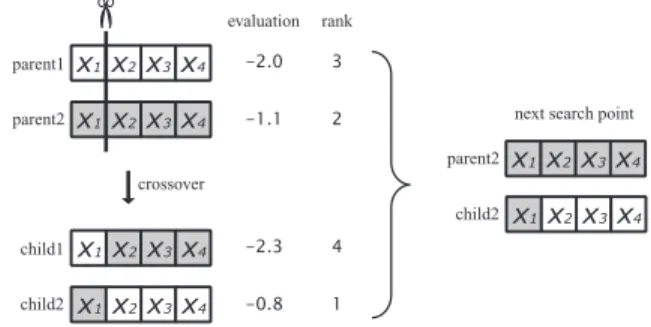
Figure 1: Simulated annealing using genetic crossover In the genetic crossover, we randomly select two individuals as parents and generate two children by genetic crossover. The genetic crossover is shown in Figure 2. An individual consists of design variables and the design variables are real numbers. Therefore, the crossover is only performed between the variables.

In the operation of genetic crossover, selection is also performed. After the crossover, there are two parents and two children. Then the two individuals that have higher evaluation values are selected. These two individuals become the next searchingpoints. While SA requires high computational costs, particularly in continuous problems, this operation reduces the computational cost.

SAs in continuous problems need deﬁnitions of the neighborhood and terminal condition. The neighborhood and acceptance criteria are explained in sections

crossover parent2

child2

next search point

x² x¹ x³x⁴

parent1 x¹x² x³x⁴

child1 x¹x²x³x⁴ x² x¹ x³x⁴

child2 x¹x² x³x⁴

parent2 x¹ x²x³x⁴

evaluation

-2.3 -1.1

-0.8 -2.0

rank

4 2

1 3

Figure 2: Crossover

3.2 and 3.3, respectively. In this paper, Metropolis criterion is used as the acceptance criterion and the exponential annealingTk+1= 0.93·Tk, wherek is the generation, is used as the cooling schedule.

3.2 Neighbourhood

In SAs, the neighborhood of the present searching point should be defined in order to find the next searchingpoint. However, it is difficult to determine the neighborhood to search efficiently, especially in continuous problems. In this paper, Corana’s algorithm is used to define the neighborhood. Corana proposes the SAs algorithm have an adjusting neighborhood range[7]. This algorithm adjusts the neighborhood range to keep the acceptance ratio to 50%for an effective search.

3.3 Termination Condition

In SA, there are several methods for terminal condi- tions. SA algorithm accepts not only improvement solutions but also worse solutions. Therefore, when the annealingtime is used as the terminal condition, the ﬁnal solution cannot be the best solution in a simulation. Furthermore, it is very diﬃcult to know the optimum annealingtimes. In this paper, we do not use an annealingtime as a terminal condition, but the movement of solution as a terminal condition. It is possible to control quality of solutions. With this terminal condition, annealingdoes not stop in the middle of a search.

4 Numerical Examples

4.1 Comparison between PSA/GAc and SA using other GA operations

In the proposed algorithm, crossover is used for exchanging the information between individuals. Is this operation best for exchanging the information? To an- swer this question, other operations that can be used in SA and are compared to PSA/GAc. These operations are explained as follows;

• PSA usingElite Selection (elitePSA): The best individual that had the highest ﬁtness value is copied to the other processes and these copies are used as the next searchingpoints.

(3)

• PSA usingRoulette Selection (roulettePSA): The next searchingpoints are determined randomly by Roulette Selection. In Roulette Selection, the individual that has the higher value can be selected with high probability.

• PSA usingRoulette Selection includingElite(e- roulettePSA): The next searchingpoints are determined by Roulette Selection but the individual that has the highest ﬁtness value will be one of the next points.

4.1.1 Test Functions

Rastrigin function (fRa) which has many local minima in global area and Griewank function (f_Gr) which has many local minima in a local area are used as continuous optimization test problems. These functions are shown as follows;

f_Ra = 10n+

n

i=1

(x²_i −10 cos(2πx_i)) (2) fmin= 0, [xi= 0], n= 2

fGr = 1 +

n

i=1

x²_i 4000−ⁿ

i=1

(cos(√xi

i)) (3) f_min= 0, [x_i= 0], n= 2

Generally, GAs can find the optimum solution of the Rastrigin function easily. On the other hand, while SAs can find the optimum solution of the Griewank function easily, it is difficult to find the optimum solution with GAs.

In the followingnumerical examples, the simulation is terminated when the value of the solution does not change more than 1.0e-4 for 100 generations. There- fore, if the solution has a value smaller than 1.0e-4 , it can be said that a good solution is derived.

4.1.2 Parameter

The parameters used in the numerical examples are summarized in Table 1(value1). All results are the average of 10 trials. The initial temperature was chosen through preparative experiments.

Table 1: Parameter of parallel SAs

parameter value 1 value 2

Population size 20, 200 400, 600

Initial temperature 5, 10, 20, 30 5, 10, 20, 30

Cooling rate 0.93 0.93

Communication interval 32 32

Neighborhood adjustment interval 8 8

4.1.3 Analysis of Results

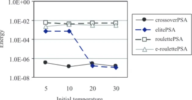
Figure 3 is the result of the Rastrigin function with 20 population on each parallel SA (PSA). In Figure 3, the energy is equal to the value of the solution. PSA/GAc (crossoverPSA) always got a good solution and was not aﬀected by the initial temperature. On the other hand, other three PSAs did not get good solutions.

Energy

crossoverPSA elitePSA roulettePSA e-roulettePSA

1.0E-08 1.0E-06 1.0E-04 1.0E-02 1.0E+00

5 10 20 30

Initial temperature

Figure 3: Results of Rastrigin function (population size 20)

In the case of 200 population, there are no diﬀer- ences between PSAs. All PSAs got good solutions.

Figure 4 and Figure 5 are the results of the Griewank function with 20 and 200 population, respectively. In Figure 4, it can be said that the results of PSA/GAc were slightly better than those of other PSAs. However, there were no signiﬁcant dif- ferences between PSAs. In the case of 200 population that is shown in Figure 5, there are diﬀerences between PSAs. PSA usingRoulette Selection and PSA usingRoulette Selection includingElite never found a good solution and PSA using Elite Selection only found good solutions at the initial temperatures of 20 and 30. PSA/GAc (crossoverPSA) found good solutions with any initial temperature.

Energy

1.0E-08 1.0E-06 1.0E-04 1.0E-02 1.0E+00

5 10 20 30

Initial temperature

Figure 4: Results of Griewank function (population size 20)

Energy

1.0E-08 1.0E-06 1.0E-04 1.0E-02 1.0E+00

5 10 20 30

Initial temperature

Figure 5: Results of Griewank function (population size 200)

The Griewank function has only one peak in the function landscape from a global view. However, it has many local minimums from a local view. Therefore,

(4)

in the case of the small number of population, the searchingpoint is trapped at the local minimum and the global optimum solution cannot be found. Because of this reason, the larger number of population needs to derive a better solution in the Griewank function.

These results show that amongPSAs usingGA operations, PSA usingGenetic Crossover is the most effective. PSA usingElite Selection also has eﬀective searchingability, but the possibility of reachinga good solution is lower than that of PSA/GAc. Therefore, it can be said that the searchingability of PSA using Elite Selection is lower than that of PSA/GAc.

4.2 Searching ability of PSA/GAc

In the numerical examples in Section4.1, we found that Parallel Simulated AnnealingusingGenetic Crossover is more eﬀective, compared to PSAs with other operations. In this section, PSA/GAc is compared to the Distributed Genetic Algorithm (DGA) and Sequential Simulated Annealing(SSA) through numerical examples.

4.2.1 Test Functions

Rastrigin function, Griewank function and Rosenbrock function are used as continuous optimization test problems. These functions are explained as follows;

fRa = 10n+

n

i=1

(x²_i −10 cos(2πxi)) (4) f_min= 0, [x_i= 0], n= 10,30 fGr = 1 +

n

i=1

x²_i 4000−

n i=1

(cos(√xi

i)) (5) fmin= 0, [xi= 0], n= 10,30 fRo =

n−1 i=1

[100(xi+1−x²_i)²+ (xi−1)²] (6) fmin= 0, [xi= 1], n= 10,30 The dimensions are equal to 10 and 30. We retain the deﬁnition of a good solution from Section 4.1.1.

4.2.2 Parameter

The parameters are summarized in Table 1(value2).

The results that are shown in the followingsections were the average of 10 trials. The initial temperatures were derived from preliminary experiments.

4.2.3 Searching ability of PSA/GAc

In Figure 6, the results of a 10 dimension Rastrigin function with PSA/GAc are shown. In the ﬁgure, (a) is the case of 400 population, and (b) is the case of 600 population. ’Average’ means the average of 10 trials,

’best’ means the best solution of 10 trials, and ’average(good solutions)’ means the average of the good results. The values of bar graph express the number of good solutions in 10 trials.

Figure 6 shows that PSA/GAc can reach the good solution with high probability, even if the problem has

10 dimensions. In the case of a 400 population, ﬁgure (a) shows that the good solutions were derived with any initial temperature and an adequate search was performed.

The results of the 30 dimension Rastrigin function problem are shown in Figure 7. Figure 7 shows that good solutions were not derived in the case of a 30 dimension Rastrigin function. SAs are not good at findingsolutions in a problem, such as the Rastrigin function, whose function landscape has many local op- tima in a global view. By comparing figures (a) and (b), it becomes apparent that the probability of finding a good solution to a problem with a large population size is higher than the probability of finding a solution to a problem with a small population size.

1.0E-06 1.0E-05 1.0E-04 1.0E-03 1.0E-02 1.0E-01 1.0E+00

5 10 20 30

0 2 4 6 8 10

1.0E-06 1.0E-05 1.0E-04 1.0E-03 1.0E-02 1.0E-01 1.0E+00

5 10 20 30

0 2 4 6 8 10

Energy Number of correct answers

Initial temperature

(a) population size 400

Number of correct answers

Energy

Initial temperature

(b) population size 600

average best average(good solutions)

correct answers

Figure 6: Results of 10 dimension Rastrigin function

1.0E-05 1.0E-04 1.0E-03 1.0E-02 1.0E-01 1.0E+00 1.0E+01

5 10 20 30

0 2 4 6 8 10

1.0E-05 1.0E-04 1.0E-03 1.0E-02 1.0E-01 1.0E+00 1.0E+01

5 10 20 30

0 2 4 6 8 10

Initial temperature

Energy

Initial temperature

correct answers

Figure 7: Results of 30 dimension Rastrigin function Figure 8 shows the results of a 10 dimension Griewank function. In this case, good solutions were derived at any initial temperature.

Energy Number of correct answers1.0E-06

1.0E-05 1.0E-04 1.0E-03 1.0E-02 1.0E-01 1.0E+00

5 10 20 30

0 2 4 6 8 10

Initial temperature

1.0E-06 1.0E-05 1.0E-04 1.0E-03 1.0E-02 1.0E-01 1.0E+00

5 10 20 30

0 2 4 6 8 10

Energy

Initial temperature

(a) population size 400 (b) population size 600

correct answers

Figure 8: Results of 10 dimension Griewank function Figure 9 shows the results of a 30 dimension Griewank function. This ﬁgure indicates that all results were better than the results of the 10 dimension

(5)

of Griewank. The Griewank function is expressed by Eq.5, and the third term of this function is the product of each dimension. Therefore, when there are many dimensions, the ﬁrst term’s aﬀect upon the value of the object function is stronger than the other terms. For this reason, a Griewank function is easy to solve if it has many dimensions.

1.0E-06 1.0E-05 1.0E-04 1.0E-03 1.0E-02 1.0E-01 1.0E+00

5 10 20 30

0 2 4 6 8 10

1.0E-06 1.0E-05 1.0E-04 1.0E-03 1.0E-02 1.0E-01 1.0E+00

5 10 20 30

0 2 4 6 8 10

Initial temperature

Energy

Initial temperature

correct answers

Figure 9: Results of 30 dimension Griewank function Figure 10 is the result of a 10 dimension Rosenbrock function, and Figure 11 is the result of a 30 dimension Rosenbrock function. GAs are not good at ﬁnding the optimum solution to Rosenbrock functions. However, in this numerical example, PSA/GAc always derived good solutions.

1.0E-10 1.0E-08 1.0E-06 1.0E-04 1.0E-02 1.0E+00

5 10 20 30

0 2 4 6 8 10

1.0E-10 1.0E-08 1.0E-06 1.0E-04 1.0E-02 1.0E+00

5 10 20 30

0 2 4 6 8 10

Initial temperature

Energy

Initial temperature

correct answers

Figure 10: Results of 10 dimension Rosenbrock function

1.0E-10 1.0E-08 1.0E-06 1.0E-04 1.0E-02 1.0E+00

5 10 20 30

0 2 4 6 8 10

1.0E-10 1.0E-08 1.0E-06 1.0E-04 1.0E-02 1.0E+00

5 10 20 30

0 2 4 6 8 10

Initial temperature

Energy

Initial temperature

correct answers

Figure 11: Results of 30 dimension Rosenbrock function

4.2.4 Comparison between PSA/GAc and Se- quential SA

In order to verify the searchingability of PSA/GAc, we compared PSA/GAc and Sequential Simulated An- nealing(SSA). In PSA/GAc, the solution was derived with 8000 generations with 400 population. Then, we deﬁne the SSA-longcompute SSA for 3200000 (8000

generations * 400 population). We deﬁne SSA-short to compute SSA for 8000 generations for 400 times.

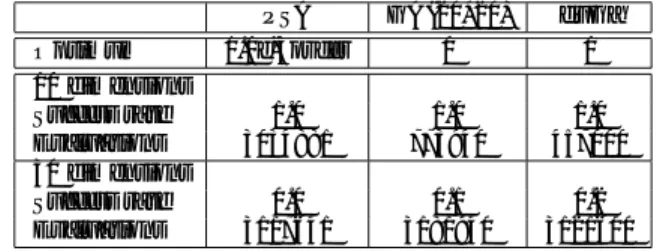
The results were compared to those of PSA/GAc. The initial temperatures were 10 in each algorithm. All results are the average of 10 trials. Table 2 is the results of Rastrigin function. In the case of 10 dimensions, PSA/GAc reached a good solution in all 10 trials. On the other hand, the two types of SSAs did not reach good solutions at all. In the case of 30 dimensions, both PGA/GAc and SSA did not reach good solutions. However, the solution values of PGA/GAc were better than those of the SSA.

Table 2: Comparison between PSA/GAc and sequential SA (Rastrigin function)

PSA SSA-long SSA-short 10 dimensions

Solution 7.64e-6 30.0 25.2

Success rate 1.0 0.0 0.0

30 dimensions

Solution 6.67 226 216

Table 3 shows the results of the Griewank function.

The Sequential SA did not reach a good solution in both the 10 dimension and the 30 dimension Rastri- gin functions. However, PSA/GAc reached the good solution with high probability.

Table 3: Comparison between PSA/GAc and sequential SA (Griewank function)

Solution 7.49e-4 3.78 0.273

30 dimensions

Solution 4.13e-5 0.459 0.592

Table 4 is the result of the Rosenbrock function. It is obvious that the results of PSA/GAc are superior to those of simple SA. This result is also derived from the results of the Griewank function test. From Table 3 and Table 4, we can find that SSA cannot find good solutions, even when the annealingtime is large. It is clear that PSA/GAc is more effective than SSA.

Table 4: Comparison between PSA/GAc and sequential SA (Rosenbrock function)

Solution 2.60e-8 1.92e-3 2.09e-3

30 dimensions

Solution 4.03e-8 1.48e-3 2.59e-3

4.2.5 Comparison between PSA/GAc and Distributed GA

In this Section, PSA/GAc is compared to the distributed genetic algorithm (DGA) and dual individual GA (DuGA). The population size, the number of

(6)

bits and the terminal condition were set up as follows:

Population size of PSA/GAc was 400, and the population of DGA and DuGA was 400 (20 individuals * 20 islands) and 400(2 individuals *200 islands), respectively. The simulation of PSA/GAc was terminated within 8000 generations and the DGA and DuGA were also terminated within 8000 generations. In each algorithm, if the optimum solution was found, the simulation was terminated before 8000 generations. The bit stringof GA was 30 per dimension. Table 5, Table 6, and Table 7 are the results of the Rastrigin function, Griewank function, and Rosenbrock function, respectively. The initial temperature of PSA was 10. All results are the average of 10 trials.

Table 5: Comparison between PSA/GAc and GA (Rastrigin function)

PSA GA(20*20) duGa

Optimum 1.0e-5order 0 0

10 dimensions

Evaluations 3034881 773940 457000 30 dimensions

Evaluations 3117641 3181940 3121600

From Table 6 and Table 7, it is clear that PSA/GAc can reach a good solution in the high probability even when the applied test functions pose diﬃcult problems for GAs. Therefore, PSA/SAc is suitable for problems that can be solved by SA, but pose diﬃculties for GA.

However, Table 5 shows that DGA is superior to the proposal algorithm in the problems where the GA is good at ﬁnding the solution.

Table 6: Comparison between PSA/GAc and GA (Griewank function)

PSA GA(20*20) duGa

10 dimensions

Evaluations 3118041 2922120 1819760

Table 7: Comparison between PSA/GAc and GA (Rosenbrock function)

PSA GA(20*20) duGa

10 dimensions

Evaluations 2723441 3200400 3200400

5 Conclusions

In this paper, we proposed a new algorithm of SA:

Parallel Simulated AnnealingusingGenetic Crossover

(PSA/GAc). In the proposed algorithm, there are several simple SA processes and each process is operated parallel. After some steps, the information of the searchingpoint is transferred amongthe processes. This information transformation is performed by crossover that is usually used in genetic algorithms.

Apart from the genetic crossover, there are other operations that are used in genetic algorithms for trans- formingthe information. Those are elite selection, roulette selection, and so on. The candidate operations were applied to the test functions and the results were compared with those of the proposed algorithm.

The result showed that the genetic crossover is better than the other candidate operations. Therefore, it can be concluded that the genetic crossover is effective operation for transforminginformation in parallel SAs. Through the numerical examples, the proposed algorithm was also compared to other emergent algorithms, sequential SAs and distributed GAs. It was found that the results of the proposed algorithm are superior to those of sequential SAs. It was also found that the proposed algorithm is good at finding solutions in problems that are not suited to GAs. Gen- erally, SAs are algorithms used for finding the solutions of discrete problems. However PSA usingGe- netic Crossover is effective for a variety of continuous problems.

References

[1] Bruce E. Rosen and Ryohei Nakano. Simulated annealing -basics and recent topics on simulated annealing- (in japanese). Proceeding of Japanese Society for Arti- ficial Intelligence, Vol. 9, No. 3, 1994.

[2] E. H. L. Aarts and J. H. M. Korst.Simulated Annealing and Boltzmann Machines. John Wiley＆Sons, 1989.

[3] Hajime Kita. Simulated annealing (in japanese). Pro- ceeding of Japan Society for Fuzzy Theory and Systems, Vol. 9, No. 6, 1997.

[4] Kenso Konishi, Kazuo Taki, and Kouichi Kimura. Tem- perature parallel simulated annealing algorithm and its evaluation. Transaction of Information Processing So- ciety of Japan, Vol. 36, No. 4, pp. 797–807, 4 1995.

[5] S. W. Mahfoud and D. E. Goldberg. A genetic algorithm for parallel simulated annealing. Parallel Prob- lem Solving from Nature 2, pp. 301–310, 1992.

[6] Naoki Mori, Junji Yoshida, and Hajime Kita. Sugges- tion of thermodynamical selection rule in genetic algorithm (in japanese). Transaction of Institute of Sys- tems, Control and Information Engineers, Vol. 9, No. 2, pp. 82–90, 1996.

[7] A. Corana, M. Marhesi, C. Martini, and S. Ridella.

Minimizing multimodal functions of continuous variables with the ’simulated annealing’ algorithm. ACM Trans. on Mathematical Sortware, Vol. 13, No. 3, pp.

262–280, 1978.

(7)

Proceedings of the IASTED International Confer- ence PARALLEL AND DISTRIBUTED COMPUT- ING AND SYSMTEMS November 6-9, 2000, Las Ve- gas, Nevada USA pp. 139-144