Econometrics II

Econometrics II

(Wed., 8:50-10:20)

Room # 509 ( ^{法経大学院総合研究棟} )

• The prerequisite of this class is knowledge about Econometrics I (last semester)

and Econometrics (undergraduate level).

TA Session (by Mr. Kinoshita):

From Oct. 9, 2013 Wed., 13:00 - 14:30

Room # 505 (

)

Content: Matrix Algebra

Econometrics (Undergraduate Course) Mon., 8:50-10:20 ( ^基礎工 B401) Fri., 8:50-10:20 ( ^基礎工 B401)

• If you have not taken Econometrics in undergraduate level, attend the above class.

• Textbook:

(

)

1 Regression Analysis ( ^回帰分析 )

1.1 Setup of the Model

When (x ₁ , y ₁ ), (x ₂ , y ₂ ), · · · , (x _n , y _n ) are available, suppose that there is a linear rela- tionship between y and x, i.e.,

y i = β 1 + β 2 x i + u i , (1) for i = 1 , 2 , · · · , n. x _i and y _i denote the ith observations.

−→ Single (or simple) regression model (

)

y _i is called the dependent variable (

) or the explained variable (

), while x i is known as the independent variable (

) or the explanatory (or explaining) variable (

).

β 1 = Intercept (

), β 2 = Slope (

)

β 1 and β 2 are unknown parameters (

) to be estimated.

β 1 and β 2 are called the regression coe ffi cients (

).

u _i is the unobserved error term (

) assumed to be a random variable with mean zero and variance σ ² .

σ ² is also a parameter to be estimated.

x i is assumed to be nonstochastic (

), but y i is stochastic (

) because y _i depends on the error u _i .

The error terms u ₁ , u ₂ , · · · , u _n are assumed to be mutually independently and iden- tically distributed, which is called iid.

It is assumed that u _i has a distribution with mean zero, i.e., E(u _i ) = 0 is assumed.

Taking the expectation on both sides of (1), the expectation of y _i is represented as:

E(y i ) = E( β 1 + β 2 x i + u i ) = β 1 + β 2 x i + E(u i )

= β 1 + β 2 x i , (2)

for i = 1 , 2 , · · · , n.

Using E(y _i ) we can rewrite (1) as y _i = E(y _i ) + u _i .

(2) represents the true regression line.

Let ˆ β 1 and ˆ β 2 be estimates of β 1 and β 2 .

Replacing β 1 and β 2 by ˆ β 1 and ˆ β 2 , (1) turns out to be:

y _i = β ˆ 1 + β ˆ 2 x _i + e _i , (3) for i = 1 , 2 , · · · , n, where e _i is called the residual (

).

The residual e i is taken as the experimental value (or realization) of u i .

We define ˆy _i as follows:

ˆy i = β ˆ 1 + β ˆ 2 x i , (4)

for i = 1 , 2 , · · · , n, which is interpreted as the predicted value (

) of y _i .

(4) indicates the estimated regression line, which is di ff erent from (2).

Moreover, using ˆy _i we can rewrite (3) as y _i = ˆy _i + e _i .

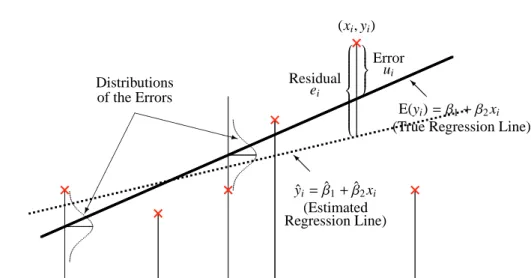
(2) and (4) are displayed in Figure 1.

Figure 1. True and Estimated Regression Lines (

)

y

XXXXX XX z Distributions

of the Errors

×

...

...

×

...

...

...

× _

 

 

 



Error u

Residual

e

(x

, y

)

×

×

×

@ @ I

ˆy

= β ˆ

+ β ˆ

x

(Estimated Regression Line)

@ @ I

E(y

) = β

+ β

x

(True Regression Line)

Consider the case of n = 6 for simplicity.

× indicates the observed data series.

The true regression line (2) is represented by the solid line, while the estimated regression line (4) is drawn with the dotted line.

Based on the observed data, β 1 and β 2 are estimated as: ˆ β 1 and ˆ β 2 .

In the next section, we consider how to obtain the estimates of β 1 and β 2 , i.e., ˆ β 1

and ˆ β 2 .

1.2 Ordinary Least Squares Estimation

Suppose that (x ₁ , y ₁ ), (x ₂ , y ₂ ), · · · , (x _n , y _n ) are available.

For the regression model (1), we consider estimating β 1 and β 2 .

Replacing β 1 and β 2 by their estimates ˆ β 1 and ˆ β 2 , remember that the residual e i is given by:

e _i = y _i − ˆy _i = y _i − β ˆ 1 − β ˆ 2 x _i . The sum of squared residuals is defined as follows:

S ( ˆ β 1 , β ˆ 2 ) =

∑ n

i = 1

e ² _i =

∑ n

i = 1

(y _i − β ˆ 1 − β ˆ 2 x _i ) ² .

It might be plausible to choose the ˆ β 1 and ˆ β 2 which minimize the sum of squared residuals, i.e., S ( ˆ β 1 , β ˆ 2 ).

This method is called the ordinary least squares estimation (

OLS).

To minimize S ( ˆ β 1 , β ˆ 2 ) with respect to ˆ β 1 and ˆ β 2 , we set the partial derivatives equal to zero:

∂ S ( ˆ β 1 , β ˆ 2 )

∂ β ˆ 1

= − 2

∑ n

i = 1

(y i − β ˆ 1 − β ˆ 2 x i ) = 0 ,

∂ S ( ˆ β 1 , β ˆ 2 )

∂ β ˆ 2

= − 2

∑ n

i = 1

x i (y i − β ˆ 1 − β ˆ 2 x i ) = 0 .

The second order condition for minimization is:

( ∂

S ( ˆ β

, β ˆ

)

∂ β ˆ

∂

S ( ˆ β

, β ˆ

)

∂ β ˆ

∂ β ˆ

∂

S ( ˆ β

, β ˆ

)

∂ β ˆ

∂ β ˆ

∂

S ( ˆ β

, β ˆ

)

∂ β ˆ

)

=

( 2n 2 ∑ n

i=1 x _i 2 ∑ _n

i = 1 x i 2 ∑ _n

i = 1 x ² _i )

should be a positive definite matrix.

The diagonal elements 2n and 2 ∑ _n

i = 1 x ² _i are positive.

The determinant:

2n 2 ∑ n

i = 1 x _i 2 ∑ _n

i = 1 x _i 2 ∑ _n

i = 1 x ² _i

= 4n

∑ n

i=1

x ² _i − 4(

∑ n

i=1

x _i ) ² = 4n

∑ n

i=1

(x _i − x) ²

is positive. = ⇒ The second-order condition is satisfied.

The first two equations yield the following two equations:

y = β ˆ 1 + β ˆ 2 x , (5)

∑ n

i = 1

x _i y _i = nx ˆ β 1 + β ˆ 2

∑ n

i = 1

x ² _i , (6)

where y = 1 n

∑ n

i = 1

y i and x = 1 n

∑ n

i = 1

x i .

Multiplying (5) by nx and subtracting (6), we can derive ˆ β 2 as follows:

β ˆ 2 =

∑ n

i = 1 x i y i − nxy

∑ _n

i = 1 x ² _i − nx ² =

∑ n

i = 1 (x i − x)(y i − y)

∑ _n

i = 1 (x i − x) ² . (7)

From (5), ˆ β 1 is directly obtained as follows:

β ˆ 1 = y − β ˆ 2 x . (8)

When the observed values are taken for y _i and x _i for i = 1 , 2 , · · · , n, we say that ˆ β 1

and ˆ β 2 are called the ordinary least squares estimates (or simply the least squares estimates,

) of β 1 and β 2 .

When y i for i = 1 , 2 , · · · , n are regarded as the random sample, we say that ˆ β 1 and ˆ β 2

are called the ordinary least squares estimators (or the least squares estimators,

) of β 1 and β 2 .

1.3 Properties of Least Squares Estimator

Equation (7) is rewritten as:

β ˆ 2 =

∑ _n

i = 1 (x i − x)(y i − y)

∑ _n

i = 1 (x _i − x) ² =

∑ _n

i = 1 (x i − x)y i

∑ _n

i = 1 (x _i − x) ² − y ∑ _n

i = 1 (x i − x)

∑ _n

i = 1 (x _i − x) ²

=

∑ n

i = 1

x _i − x

∑ _n

i = 1 (x _i − x) ² y _i =

∑ n

i = 1

ω i y _i . (9)

In the third equality,

∑ n

i = 1

(x _i − x) = 0 is utilized because of x = 1 n

∑ n

i = 1

x _i . In the fourth equality, ω i is defined as: ω i = x _i − x

∑ _n

i = 1 (x _i − x) ² .

ω i is nonstochastic because x i is assumed to be nonstochastic.

ω i has the following properties:

∑ n

i=1

ω i =

∑ n

i=1

x _i − x

∑ n

i = 1 (x _i − x) ² =

∑ n

i = 1 (x _i − x)

∑ n

i = 1 (x _i − x) ² = 0 , (10)

∑ n

i = 1

ω i x _i =

∑ n

i = 1

ω i (x _i − x) =

∑ _n

i = 1 (x _i − x) ²

∑ _n

i = 1 (x _i − x) ² = 1 , (11)

∑ n

i = 1

ω ² i =

∑ n

i = 1

( x i − x

∑ n

i=1 (x _i − x) ² ) 2

=

∑ n

i=1 (x _i − x) ² (∑ n

i = 1 (x i − x) ² ) 2 = 1

∑ n

i=1 (x _i − x) ² . (12)

The first equality of (11) comes from (10).

From now on, we focus only on ˆ β 2 , because usually β 2 is more important than β 1 in the regression model (1).

In order to obtain the properties of the least squares estimator ˆ β 2 , we rewrite (9) as:

β ˆ 2 =

∑ n

i=1

ω i y _i =

∑ n

i=1

ω i ( β 1 + β 2 x _i + u _i )

= β 1

∑ n

i=1

ω i + β 2

∑ n

i=1

ω i x _i +

∑ n

i=1

ω i u _i = β 2 +

∑ n

i=1

ω i u _i . (13)

In the fourth equality of (13), (10) and (11) are utilized.

Mean and Variance of ˆ β 2 : u ₁ , u ₂ , · · · , u _n are assumed to be mutually indepen- dently and identically distributed with mean zero and variance σ ² , but they are not necessarily normal.

Remember that we do not need normality assumption to obtain mean and variance but the normality assumption is required to test a hypothesis.

From (13), the expectation of ˆ β 2 is derived as follows:

E( ˆ β 2 ) = E( β 2 +

∑ n

i = 1

ω i u i ) = β 2 + E(

∑ n

i = 1

ω i u i )

= β 2 +

∑ n

i = 1

ω i E(u i ) = β 2 . (14)

It is shown from (14) that the ordinary least squares estimator ˆ β 2 is an unbiased estimator of β 2 .

From (13), the variance of ˆ β 2 is computed as:

V( ˆ β 2 ) = V( β 2 +

∑ n

i = 1

ω i u _i ) = V(

∑ n

i = 1

ω i u _i ) =

∑ n

i = 1

V( ω i u _i ) =

∑ n

i = 1

ω ² _i V(u _i )

= σ ²

∑ n

i = 1

ω ² _i = ∑ _n σ ²

i = 1 (x i − x) ² . (15)

The third equality holds because u 1 , u 2 , · · · , u n are mutually independent.

The last equality comes from (12).

Thus, E( ˆ β 2 ) and V( ˆ β 2 ) are given by (14) and (15).

Gauss-Markov Theorem (

): It has been discussed above that ˆ β 2 is represented as (9), which implies that ˆ β 2 is a linear estimator, i.e., linear in y _i .

In addition, (14) indicates that ˆ β 2 is an unbiased estimator.

Therefore, summarizing these two facts, it is shown that ˆ β 2 is a linear unbiased

estimator (

).

Furthermore, here we show that ˆ β 2 has minimum variance within a class of the linear unbiased estimators.

Consider the alternative linear unbiased estimator ˜ β 2 as follows:

β ˜ 2 =

∑ n

i = 1

c _i y _i =

∑ n

i = 1

( ω i + d _i )y _i ,

where c _i = ω i + d _i is defined and d _i is nonstochastic.

Then, ˜ β 2 is transformed into:

β ˜ 2 =

∑ n

i = 1

c _i y _i =

∑ n

i = 1

( ω i + d _i )( β 1 + β 2 x _i + u _i )

= β 1

∑ n

i = 1

ω i + β 2

∑ n

i = 1

ω i x _i +

∑ n

i = 1

ω i u _i + β 1

∑ n

i = 1

d _i + β 2

∑ n

i = 1

d _i x _i +

∑ n

i = 1

d _i u _i

= β 2 + β 1

∑ n

i = 1

d _i + β 2

∑ n

i = 1

d _i x _i +

∑ n

i = 1

ω i u _i +

∑ n

i = 1

d _i u _i .

Equations (10) and (11) are used in the forth equality.

Taking the expectation on both sides of the above equation, we obtain:

E( ˜ β 2 ) = β 2 + β 1

∑ n

i = 1

d i + β 2

∑ n

i = 1

d i x i +

∑ n

i = 1

ω i E(u i ) +

∑ n

i = 1

d i E(u i )

= β 2 + β 1

∑ n

i = 1

d i + β 2

∑ n

i = 1

d i x i .

Note that d _i is not a random variable and that E(u _i ) = 0.

Since ˜ β 2 is assumed to be unbiased, we need the following conditions:

∑ n

i=1

d _i = 0 ,

∑ n

i=1

d _i x _i = 0 .

When these conditions hold, we can rewrite ˜ β 2 as:

β ˜ 2 = β 2 +

∑ n

i = 1

( ω i + d _i )u _i . The variance of ˜ β 2 is derived as:

V( ˜ β 2 ) = V ( β 2 +

∑ n

i = 1

( ω i + d i )u i

) = V ( ∑ ⁿ

i = 1

( ω i + d i )u i

) =

∑ n

i = 1

V (

( ω i + d i )u i

)

=

∑ n

i = 1

( ω i + d i ) ² V(u i ) = σ ² (

∑ n

i = 1

ω ² i + 2

∑ n

i = 1

ω i d i +

∑ n

i = 1

d _i ² )

= σ ² (

∑ n

i = 1

ω ² i +

∑ n

i = 1

d _i ² ) .

From unbiasedness of ˜ β 2 , using ∑ n

i=1 d _i = 0 and ∑ n

i=1 d _i x _i = 0, we obtain:

∑ n

i = 1

ω i d _i =

∑ _n

i = 1 (x _i − x)d _i

∑ _n

i = 1 (x _i − x) ² =

∑ _n

i = 1 x _i d _i − x ∑ _n

i = 1 d _i

∑ _n

i = 1 (x _i − x) ² = 0 ,

which is utilized to obtain the variance of ˜ β 2 in the third line of the above equation.

From (15), the variance of ˆ β 2 is given by: V( ˆ β 2 ) = σ ² ∑ n i = 1 ω ² _i . Therefore, we have:

V( ˜ β 2 ) ≥ V( ˆ β 2 ) , because of ∑ n

i=1 d ² _i ≥ 0.

When ∑ n

i=1 d ² _i = 0, i.e., when d ₁ = d ₂ = · · · = d _n = 0, we have the equality: V( ˜ β 2 )

= V( ˆ β 2 ).

Thus, in the case of d ₁ = d ₂ = · · · = d _n = 0, ˆ β 2 is equivalent to ˜ β 2 .

As shown above, the least squares estimator ˆ β 2 gives us the minimum variance

linear unbiased estimator (

), or equivalently the best

linear unbiased estimator (

BLUE), which is called the

Gauss-Markov theorem (

).

Asymptotic Properties (

) of ˆ β 2 : We assume that as n goes to infinity we have the following:

1 n

∑ n

i = 1

(x _i − x) ² −→ m < ∞,

where m is a constant value. From (12), we obtain:

n

∑ n

i = 1

ω ² _i = 1

(1 / n) ∑ _n

i = 1 (x _i − x) −→ 1

m .

Note that f (x _n ) −→ f (m) when x _n −→ m, called Slutsky’s theorem (スルツキー

), where m is a constant value and f ( · ) is a function.

We show both consistency (

) of ˆ β 2 and asymptotic normality (

) of √

n( ˆ β 2 − β 2 ).

●

First, we prove that ˆ β 2 is a consistent estimator of β 2 .

[Review] Chebyshev’s inequality (

) is given by:

P( | X − µ| > ) ≤ σ ²

² , where µ = E(X) and σ ² = V(X).

[End of Review]

Replace X, E(X) and V(X) by:

β ˆ 2 , E( ˆ β 2 ) = β 2 , and V( ˆ β 2 ) = σ ²

∑ n

i=1

ω ² i = σ ²

∑ n

i = 1 (x i − x) .

Then, when n −→ ∞ , we obtain the following result:

P( | β ˆ 2 − β 2 | > ) ≤ σ ² ∑ n i=1 ω ² _i

² = σ ² n ∑ n i=1 ω ² _i

n ² −→ 0 , where ∑ n

i = 1 ω ² _i −→ 0 because n ∑ n

i = 1 ω ² _i −→ 1

m from the assumption.

Thus, we obtain the result that ˆ β 2 −→ β 2 as n −→ ∞ .

Therefore, we can conclude that ˆ β 2 is a consistent estimator (

) of β 2 .

●

Next, we want to show that √

n( ˆ β 2 − β 2 ) is asymptotically normal.

[Review] The Central Limit Theorem (

, CLT) is: for random variables X ₁ , X ₂ , · · · , X _n ,

X − E(X)

√ V(X)

=

∑ n

i = 1 X i − E( ∑ n i = 1 X i )

√ V( ∑ _n

i=1 X _i ) −→ N(0 , 1) , as n −→ ∞, where X = 1

n

∑ n

i = 1

X _i .

X ₁ , X ₂ , · · · , X _n are not necesarily iid, if V(X) is finite as n goes to infinity.

[End of Review]

Note that ˆ β 2 = β 2 + ∑ n

i=1 ω i u _i as in (13), and X _i is replaced by ω i u _i . From the central limit theorem, asymptotic normality is shown as follows:

∑ _n

i = 1 ω i u i − E( ∑ _n

i = 1 ω i u i )

√ V( ∑ n

i=1 ω i u _i ) =

∑ _n

i = 1 ω i u i

σ √∑ n

i = 1 ω ² _i = β ˆ 2 − β 2

σ/ √∑ n

i=1 (x _i − x) ² −→ N(0 , 1) , where

• E( ∑ _n

i=1 ω i u _i ) = 0,

• V( ∑ n

i = 1 ω i u i ) = σ ² ∑ n

i = 1 ω ² _i , and

• ∑ _n

i=1 ω i u _i = β ˆ 2 − β 2

are substituted in the first and second equalities.

Moreover, we can rewrite as follows:

β ˆ 2 − β 2

σ/ √∑ n

i = 1 (x i − x) ² =

√ n( ˆ β 2 − β 2 ) σ/ √

(1 / n) ∑ _n

i = 1 (x i − x) ² −→

√ n( ˆ β 2 − β 2 ) σ/ √

m −→ N(0 , 1) . Or equivalently,

√ n( ˆ β 2 − β 2 ) −→ N(0 , σ ² m ) . Thus, the asymptotic normality of √

n( ˆ β 2 − β 2 ) is shown.

Finally, replacing σ ² by its consistent estimator s ² , it is known as follows:

β ˆ 2 − β 2

s / √∑ n

i = 1 (x i − x) ² −→ N(0 , 1) , (16)

where s ² is defined as:

s ² = 1 n − 2

∑ n

i = 1

e ² _i = 1 n − 2

∑ n

i = 1

(y _i − β ˆ 1 − β ˆ 2 x _i ) ² , (17) which is a consistent and unbiased estimator of σ ² . −→ Proved later.

Thus, using (16), in large sample we can construct the confidence interval and test

the hypothesis.

Exact Distribution of ˆ β 2 : We have shown asymptotic normality of √

n( ˆ β 2 − β 2 ), which is one of the large sample properties.

Now, we discuss the small sample properties of ˆ β 2 .

In order to obtain the distribution of ˆ β 2 in small sample, the distribution of the error term has to be assumed.

Therefore, the extra assumption is that u i ∼ N(0 , σ ² ).

Writing (13), again, ˆ β 2 is represented as:

β ˆ 2 = β 2 +

∑ n

i = 1

ω i u _i .

First, we obtain the distribution of the second term in the above equation.

[Review] Note that the moment-generating function (

, MGF) is given by M( θ ) ≡ E(exp( θ X)) = exp( µθ + ¹ ₂ σ ² θ ² ) when X ∼ N( µ, σ ² ).

X ₁ , X ₂ , · · · , X _n are mutually independently distributed as X _i ∼ N( µ i , σ ² _i ) for i = 1 , 2 , · · · , n.

MGF of X _i is M _i ( θ ) ≡ E(exp( θ X _i )) = exp( µ i θ + ¹ ₂ σ ² _i θ ² ).

Consider the distribution of Y = ∑ n

i = 1 (a i + b i X i ), where a i and b i are constant.

M _y ( θ ) ≡ E(exp( θ Y)) = E(exp( θ ∑ n

i=1 (a _i + b _i X _i )))

= ∏ _n

i = 1 exp( θ a i )E(exp( θ b i X i )) = ∏ _n

i = 1 exp( θ a i )M i ( θ b i )

= ∏ n

i=1 exp( θ a _i ) exp( µ i θ b _i + ¹ ₂ σ ² _i ( θ b _i ) ² ) = exp( θ ∑ n

i=1 (a _i + b _i µ i ) + ¹ ₂ θ ² ∑ n

i=1 b ² _i σ ² _i ),

which implies that Y ∼ N( ∑ n

i=1 (a _i + b _i µ i ) , ∑ n

i=1 b ² _i σ ² _i ).

[End of Review]

Substitute a i = 0, µ i = 0, b i = ω i and σ ² _i = σ ² . Then, using the moment-generating function, ∑ n

i = 1 ω i u _i is distributed as:

∑ n

i = 1

ω i u _i ∼ N(0 , σ ²

∑ n

i = 1

ω ² i ) . Therefore, ˆ β 2 is distributed as:

β ˆ 2 = β 2 +

∑ n

i = 1

ω i u i ∼ N( β 2 , σ ²

∑ n

i = 1

ω ² i ) ,

or equivalently,

β ˆ 2 − β 2

σ √∑ n

i = 1 ω ² _i = β ˆ 2 − β 2

σ/ √∑ n

i = 1 (x i − x) ² ∼ N(0 , 1) , for any n.

Moreover, replacing σ ² by its estimator s ² defined in (17), it is known that we have:

β ˆ 2 − β 2

s / √∑ n

i = 1 (x _i − x) ² ∼ t(n − 2) ,

where t(n − 2) denotes t distribution with n − 2 degrees of freedom.

Thus, under normality assumption on the error term u _i , the t(n − 2) distribution is used for the confidence interval and the testing hypothesis in small sample.

Or, taking the square on both sides,

( β ˆ 2 − β 2

s / √∑ n

i = 1 (x _i − x) ² ) 2

∼ F(1 , n − 2) ,

which will be proved later.

Before going to multiple regression model (

),

2 Some Formulas of Matrix Algebra

1. Let A =

 







a ₁₁ a ₁₂ · · · a _1k a 21 a 22 · · · a 2k

... ... ... ...

a l1 a l2 · · · a lk

 





 = [a _{i j} ],

which is a l × k matrix, where a i j denotes ith row and jth column of A.

The transposed matrix (

) of A, denoted by A ⁰ , is defined as:

A ⁰ =

 







a ₁₁ a ₂₁ · · · a _l1 a 12 a 22 · · · a l2

... ... ... ...

a 1k a 2k · · · a lk

 





 = [a _ji ],

where the ith row of A ⁰ is the ith column of A.

2. (Ax) ⁰ = x ⁰ A ⁰ ,

where A and x are a l × k matrix and a k × 1 vector, respectively.

3. a ⁰ = a,

where a denotes a scalar.

4. ∂ a ⁰ x

∂ x = a,

where a and x are k × 1 vectors.

5. ∂ x ⁰ Ax

∂ x = (A + A ⁰ )x,

where A and x are a k × k matrix and a k × 1 vector, respectively.

Especially, when A is symmetric,

∂ x ⁰ Ax

∂ x = 2Ax.

6. Let A and B be k × k matrices, and I _k be a k × k identity matrix (

) (one in the diagonal elements and zero in the other elements).

When AB = I _k , B is called the inverse matrix (

) of A, denoted by B = A ^{− 1} .

That is, AA ^{− 1} = A ^{− 1} A = I _k .

7. Let A be a k × k matrix and x be a k × 1 vector.

If A is a positive definite matrix (

), for any x except for x = 0 we have:

x ⁰ Ax > 0 .

If A is a positive semidefinite matrix (

), for any x except for x = 0 we have:

x ⁰ Ax ≥ 0 .

If A is a negative definite matrix (

), for any x except for x = 0 we have:

x ⁰ Ax < 0 .

If A is a negative semidefinite matrix (

), for any x except for x = 0 we have:

x ⁰ Ax ≤ 0 .

Trace, Rank and etc.: A : k × k, B : n × k, C : k × n.

1. The trace (

) of A is: tr(A) =

∑ k

i = 1

a _ii , where A = [a _{i j} ] .

2. The rank (

) of A is the maximum number of linearly indepen- dent column (or row) vectors of A, which is denoted by rank(A).

3. If A is an idempotent matrix (

), A = A ² .

4. If A is an idempotent and symmetric matrix, A = A ² = A ⁰ A .

5. A is idempotent if and only if the eigen values of A consist of 1 and 0.

6. If A is idempotent, rank(A) = tr(A) .

7. tr(BC) = tr(CB)

Distributions in Matrix Form:

1. Let X, µ and Σ be k × 1, k × 1 and k × k matrices.

When X ∼ N( µ, Σ ), the density function of X is given by:

f (x) = 1

(2 π ) ^{k / 2} |Σ| exp (

− 1

2 (x − µ ) ⁰ Σ ⁻¹ (x − µ ) )

.

E(X) = µ and V(X) = E (

(X − µ )(X − µ ) ⁰ )

= Σ The moment-generating function: φ ( θ ) = E (

exp( θ ⁰ X) )

= exp( θ ⁰ µ + ¹ ₂ θ ⁰ Σθ )

2. If X ∼ N( µ, Σ ), then (X − µ ) ⁰ Σ ⁻¹ (X − µ ) ∼ χ ² (k).

Note that X ⁰ X ∼ χ ² (k) when X ∼ N(0 , I _k ).

3. X: n × 1, Y: m × 1, X ∼ N( µ x , Σ x ), Y ∼ N( µ y , Σ y ) X is independent of Y, i.e., E (

(X − µ x )(Y − µ y ) ⁰ )

= 0 in the case of normal random variables.

(X − µ x ) ⁰ Σ ⁻ x ¹ (X − µ x ) / n

(Y − µ y ) ⁰ Σ ⁻ y ¹ (Y − µ y ) / m ∼ F(n , m)

4. If X ∼ N(0 , σ ² I _n ) and A is a symmetric idempotent n × n matrix of rank G, then X ⁰ AX /σ ² ∼ χ ² (G).

Note that X ⁰ AX = (AX) ⁰ (AX) and rank(A) = tr(A) because A is idempotent.

5. If X ∼ N(0 , σ ² I _n ), A and B are symmetric idempotent n × n matrices of rank G and K, and AB = 0, then

X ⁰ AX G σ ²

/ X ⁰ BX

K σ ² = X ⁰ AX / G

X ⁰ BX / K ∼ F(G , K) .

3 Multiple Regression Model ( ^{重回帰モデル} )

Up to now, only one independent variable, i.e., x _i , is taken into the regression model.

In this section, we extend it to more independent variables, which is called the

multiple regression model (

).

We consider the following regression model:

y i = β 1 x i , 1 + β 2 x i , 2 + · · · + β k x i , k + u i

= (x _i,1 , x _i,2 , · · · , x _i,k )

 







β 1

β 2

...

β k

 





 + u _i

= x _i β + u _i , for i = 1 , 2 , · · · , n,

where x _i and β denote a 1 × k vector of the independent variables and a k × 1 vector

of the unknown parameters to be estimated, which are represented as:

x _i = (x _{i , 1} , x _{i , 2} , · · · , x _{i , k} ) , β =

 







β 1

β 2

...

β k

 





 .

x _{i, j} denotes the ith observation of the jth independent variable.

The case of k = 2 and x _{i , 1} = 1 for all i is exactly equivalent to (1).

Therefore, the matrix form above is a generalization of (1).

Writing all the equations for i = 1 , 2 , · · · , n, we have:

y 1 = β 1 x 1 , 1 + β 2 x 1 , 2 + · · · + β k x 1 , k + u 1 = x 1 β + u 1 , y 2 = β 1 x 2 , 1 + β 2 x 2 , 2 + · · · + β k x 2 , k + u 2 = x 2 β + u 2 ,

...

y n = β 1 x n , 1 + β 2 x n , 2 + · · · + β k x n , k + u n = x n β + u n ,

which is rewritten as:

 







y ₁ y ₂ ...

y _n

 





 =

 







x _1,1 x _1,2 · · · x _1,k x _{2 , 1} x _{2 , 2} · · · x _{2 , k} ... ... ... ...

x _{n , 1} x _{n , 2} · · · x _{n , k}

 







 







β 1

β 2

...

β k

 





 +

 







u ₁ u ₂ ...

u _n

 







=

 







x ₁ x ₂ ...

x _n

 





 β +

 







u ₁ u ₂ ...

u _n

 





 .

Again, the above equation is compactly rewritten as:

y = X β + u , (18)

where y, X and u are denoted by:

y =

 







y ₁ y ₂ ...

y _n

 





 , X =

 







x _1,1 x _1,2 · · · x _1,k x _{2 , 1} x _{2 , 2} · · · x _{2 , k} ... ... ... ...

x _{n , 1} x _{n , 2} · · · x _{n , k}

 





 =

 







x ₁ x ₂ ...

x _n

 





 , u =

 







u ₁ u ₂ ...

u _n

 





 .

Utilizing the matrix form (18), we derive the ordinary least squares estimator of β ,

denoted by ˆ β .

In (18), replacing β by ˆ β , we have the following equation:

y = X ˆ β + e , where e denotes a n × 1 vector of the residuals.

The ith element of e is given by e i .

The sum of squared residuals is written as follows:

S ( ˆ β ) =

∑ n

i=1

e ² _i = e ⁰ e = (y − X ˆ β ) ⁰ (y − X ˆ β ) = (y ⁰ − β ˆ ⁰ X ⁰ )(y − X ˆ β )

= y ⁰ y − y ⁰ X ˆ β − β ˆ ⁰ X ⁰ y + β ˆ ⁰ X ⁰ X ˆ β = y ⁰ y − 2y ⁰ X ˆ β + β ˆ ⁰ X ⁰ X ˆ β.

In the last equality, note that ˆ β ⁰ X ⁰ y = y ⁰ X ˆ β because both are scalars.

To minimize S ( ˆ β ) with respect to ˆ β , we set the first derivative of S ( ˆ β ) equal to zero, i.e.,

∂ S ( ˆ β )

∂ β ˆ = − 2X ⁰ y + 2X ⁰ X ˆ β = 0 .

Solving the equation above with respect to ˆ β , the ordinary least squares estimator (OLS,

) of β is given by:

β ˆ = (X ⁰ X) ^{− 1} X ⁰ y . (19)

Thus, the ordinary least squares estimator is derived in the matrix form.

(*) Remark

The second order condition for minimization:

∂ ² S ( ˆ β )

∂ β∂ ˆ β ˆ ⁰ = 2X ⁰ X is a positive definite matrix.

Set c = Xd.

For any d , 0, we have c ⁰ c = d ⁰ X ⁰ Xd > 0.

Now, in order to obtain the properties of ˆ β such as mean, variance, distribution and so on, (19) is rewritten as follows:

β ˆ = (X ⁰ X) ^{− 1} X ⁰ y = (X ⁰ X) ^{− 1} X ⁰ (X β + u) = (X ⁰ X) ^{− 1} X ⁰ X β + (X ⁰ X) ^{− 1} X ⁰ u

= β + (X ⁰ X) ^{− 1} X ⁰ u . (20)

Taking the expectation on both sides of (20), we have the following:

E( ˆ β ) = E( β + (X ⁰ X) ^{− 1} X ⁰ u) = β + (X ⁰ X) ^{− 1} X ⁰ E(u) = β, because of E(u) = 0 by the assumption of the error term u _i .

Thus, unbiasedness of ˆ β is shown.

The variance of ˆ β is obtained as:

V( ˆ β ) = E(( ˆ β − β )( ˆ β − β ) ⁰ ) = E (

(X ⁰ X) ^{− 1} X ⁰ u((X ⁰ X) ^{− 1} X ⁰ u) ⁰ )

= E((X ⁰ X) ^{− 1} X ⁰ uu ⁰ X(X ⁰ X) ^{− 1} ) = (X ⁰ X) ^{− 1} X ⁰ E(uu ⁰ )X(X ⁰ X) ^{− 1}

= σ ² (X ⁰ X) ^{− 1} X ⁰ X(X ⁰ X) ^{− 1} = σ ² (X ⁰ X) ^{− 1} .

The first equality is the definition of variance in the case of vector.

In the fifth equality, E(uu ⁰ ) = σ ² I _n is used, which implies that E(u ² _i ) = σ ² for all i and E(u i u j ) = 0 for i , j.

Remember that u ₁ , u ₂ , · · · , u _n are assumed to be mutually independently and identi-

cally distributed with mean zero and variance σ ² .

Under normality assumption on the error term u, it is known that the distribution of β ˆ is given by:

β ˆ ∼ N( β, σ ² (X ⁰ X) ^{− 1} ) . Proof:

First, when X ∼ N( µ, Σ ), the moment-generating function, i.e., φ ( θ ), is given by:

φ ( θ ) ≡ E (

exp( θ ⁰ X) )

= exp (

θ ⁰ µ + 1

2 θ ⁰ Σθ )

θ u : n × 1, u: n × 1, θ _β : k × 1, β ˆ : k × 1 The moment-generating function of u, i.e., φ u ( θ u ), is:

φ u ( θ u ) ≡ E (

exp( θ ⁰ u u) )

= exp ( σ ² 2 θ u ⁰ θ u

) ,

which is N(0 , σ ² I _n ).

The moment-generating function of ˆ β , i.e., φ _β ( θ _β ), is:

φ β ( θ β ) ≡ E (

exp( θ _β ⁰ β ˆ ) )

= E (

exp( θ ⁰ _β β + θ ⁰ _β (X ⁰ X) ^{− 1} X ⁰ u) )

= exp( θ ⁰ _β β )E (

exp( θ ⁰ _β (X ⁰ X) ^{− 1} X ⁰ u) )

= exp( θ _β ⁰ β ) φ u

( θ ⁰ _β (X ⁰ X) ^{− 1} X ⁰ )

= exp( θ ⁰ _β β ) exp ( σ ²

2 θ _β ⁰ (X ⁰ X) ^{− 1} θ β

) = exp (

θ ⁰ _β β + σ ²

2 θ ⁰ _β (X ⁰ X) ^{− 1} θ β

) ,

which is equivalent to the normal distribution with mean β and variance σ ² (X ⁰ X) ⁻¹ .

Note that θ u = X(X ⁰ X) ^{− 1} θ β . QED

Taking the jth element of ˆ β , its distribution is given by:

β ˆ j ∼ N( β j , σ ² a _{j j} ) , i.e.,

β ˆ j − β j

σ √

a j j ∼ N(0 , 1) , where a _{j j} denotes the jth diagonal element of (X ⁰ X) ⁻¹ .

Replacing σ ² by its estimator s ² , we have the following t distribution:

β ˆ j − β j

s √ a _{j j} ∼ t(n − k) ,

where t(n − k) denotes the t distribution with n − k degrees of freedom.

s ² is taken as follows:

s ² = 1 n − k

∑ n

i = 1

e ² _i = 1

n − k e ⁰ e = 1

n − k (y − X ˆ β ) ⁰ (y − X ˆ β ) , which leads to an unbiased estimator of σ ² .

Proof:

Substitute y = X β + u and ˆ β = β + (X ⁰ X) ^{− 1} X ⁰ u into e = y − X ˆ β . e = y − X ˆ β = X β + u − X( β + (X ⁰ X) ^{− 1} X ⁰ u)

= u − X(X ⁰ X) ^{− 1} X ⁰ u = (I _n − X(X ⁰ X) ^{− 1} X ⁰ )u

I _n − X(X ⁰ X) ⁻¹ X ⁰ is idempotent and symmetric, because we have:

(I n − X(X ⁰ X) ^{− 1} X ⁰ )(I n − X(X ⁰ X) ^{− 1} X ⁰ ) = I n − X(X ⁰ X) ^{− 1} X , ⁰ (I n − X(X ⁰ X) ^{− 1} X ⁰ ) ⁰ = I n − X(X ⁰ X) ^{− 1} X ⁰ .

s ² is rewritten as follows:

s ² = 1

n − k e ⁰ e = 1

n − k ((I _n − X(X ⁰ X) ⁻¹ X ⁰ )u) ⁰ (I _n − X(X ⁰ X) ⁻¹ X ⁰ )u

= 1

n − k u ⁰ (I _n − X(X ⁰ X) ^{− 1} X ⁰ ) ⁰ (I _n − X(X ⁰ X) ^{− 1} X ⁰ )u

= 1

n − k u ⁰ (I _n − X(X ⁰ X) ^{− 1} X ⁰ )u

Take the expectation of u ⁰ (I _n − X(X ⁰ X) ⁻¹ X ⁰ )u and note that tr(a) = a for a scalar a.

E(s ² ) = 1 n − k E (

tr (

u ⁰ (I _n − X(X ⁰ X) ⁻¹ X ⁰ )u ))

= 1 n − k E (

tr (

(I _n − X(X ⁰ X) ⁻¹ X ⁰ )uu ⁰ ))

= 1 n − k tr (

(I n − X(X ⁰ X) ^{− 1} X ⁰ )E(uu ⁰ ) )

= 1

n − k σ ² tr (

(I n − X(X ⁰ X) ^{− 1} X ⁰ )I n

)

= 1

n − k σ ² tr(I _n − X(X ⁰ X) ^{− 1} X ⁰ ) = 1

n − k σ ² (tr(I _n ) − tr(X(X ⁰ X) ^{− 1} X ⁰ ))

= 1

n − k σ ² (tr(I n ) − tr((X ⁰ X) ^{− 1} X ⁰ X)) = 1

n − k σ ² (tr(I n ) − tr(I k ))

= 1

n − k σ ² (n − k) = σ ²

−→ s ² is an unbiased estimator of σ ² .

Note that we do not need normality assumption for unbiasedness of s ² .

Trace (

):

1. A: n × n, tr(A) = ∑ _n

i = 1 a ii , where a i j denotes an element in the ith row and the jth column of a matrix A.

2. a: scalar (1 × 1), tr(a) = a

3. A: n × k, B: k × n, tr(AB) = tr(BA)

4. tr(X(X ⁰ X) ^{− 1} X ⁰ ) = tr((X ⁰ X) ^{− 1} X ⁰ X) = tr(I _k ) = k

5. When X is a vector of random variables, E(tr(X)) = tr(E(X))

Under normality assumption for u, the distribution of s ² is:

(n − k)s ²

σ ² = u ⁰ (I _n − X(X ⁰ X) ^{− 1} X ⁰ )u

σ ² ∼ χ ² (tr(I _n − X(X ⁰ X) ^{− 1} X ⁰ ))

Note that tr(I _n − X(X ⁰ X) ^{− 1} X ⁰ ) = n − k, because tr(I _n ) = n

tr(X(X ⁰ X) ^{− 1} X ⁰ ) = tr((X ⁰ X) ^{− 1} X ⁰ X) = tr(I _k ) = k