Wealth Inequality and Conditionality in Cash Transfers : A Politico‑Economic Approach
著者 KITAURA Koji, MIYAZAWA Kazutoshi
出版者 Institute of Comparative Economic Studies, Hosei University
journal or
publication title
Working Paper
volume 215
page range 1‑36
year 2019‑11‑30
URL http://hdl.handle.net/10114/00022487
1
Wealth Inequality and Conditionality in Cash Transfers: A Politico-Economic Approach
Koji Kitaura a,*
aFaculty of Social Sciences, Hosei University, 4342 Aihara, Machida, Tokyo 194-0298, Japan
Kazutoshi Miyazawab
bFaculty of Economics, Doshisha University, Kamigyo, Kyoto 602-8580, Japan
Abstract
We present a model that offers an explanation whether a condition is attached to cash transfers affects the elimination of child labor, taking into account wealth heterogeneity (especially land).
The cash transfer program designs (conditional vs. unconditional) is determined through a political process. We show that when wealth distribution is left-skewed, median voters support conditional cash transfers, which reduces child labor. Unconditional cash transfers enjoy political support when the wealth distribution is less skewed; however, child labor remains. Our cross-country estimation confirms that countries with a greater wealth inequality are adopted conditional cash transfer in a number of developing and transition economies. The effects of sibling differences on child labor and cash transfer programs are also examined.
Keywords: Conditional Cash Transfer; Child Labor; Wealth Inequality JEL Classification: D13, J20, O12
* Corresponding author.
E-mail addresses: [email protected] (K. Kitaura).
2 1. Introduction
Over the last several decades, the governments of developing and transitional countries have implemented the cash transfer (CT) programs that focus on poverty and inequality alleviation.
It is well-known that CT programs may be conditional or unconditional; conditional cash transfers (CCTs) transfer cash to poor households on the condition that the recipients meet certain requirements, while unconditional cash transfers (UCTs) provide benefits to all eligible beneficiaries. Since Mexico’s pioneering PROGRESA (renamed Oportunidades) was launched in 1997, CCTs have become one of the most popular programs for reducing inequality, especially in the very unequal countries in Latin America (Fiszbein and Schady, 2009).1 Today, CCTs have become the main social assistance intervention in developing and transitional economies, being implemented in 64 countries as of 2014 (World Bank, 2015). Despite the success of CCTs in some Latin America and the Caribbean, many CT programs in sub-Saharan Africa in force since 2000 have been unconditional, so as to focus on extremely poor.2 Gaader (2012) points out that UCTs have been adopted in sub-Saharan Africa rather than CCTs due to the lack of public services in the poor areas of several African countries.3 The debate over whether conditionality should be attached to cash transfers has continued to be one of the most important issues in developing economies (see, for example, Schubert and Slater, 2006; Baird et al., 2011; Davis et al., 2012; Gaader, 2012; Garcia et al., 2012). Behrman and Skoufias (2006) suggest that CCTs are not necessarily superior to UCTs although they demonstrate the positive impacts of the CCTs on poverty and human development outcomes.4 Experimental evidence from Malawi has also shows that conditions may be relevant for certain, but not all, cash transfers directly comparing the effects of UCTs to CCTs (Baird et al., 2011).5 Recently, using data from 75 reports that cover 35 different studies, Baird et al., (2014) find that the effects of CCTs are always larger than those of UCTs in relation to school enrolment and attendance, but
1 Fiszbein and Schady (2009) provide the first comprehensive report of CCTs, which have become popular in developing countries over the last decade. This review confirms with much evidence that CCTs have been effective in reducing poverty and expanding access to education and health services in developing countries.
2 Garcia et al., (2012) mention that CCTs also have also relatively increased, reaching in 13 countries in 2010 (p.46). They report that 5 countries have only had CCTs, and 21 countries have only had UCTs. In addition, they note that 9 countries have had both CCTs and UCTs.
3 See, several papers, including Gaader (2012) in “Conditional versus unconditional cash: a commentary” in the Journal of Development Effectiveness 4 (1), 2012.
4 Using the data from the PROGRESA randomized experiment, Schultz (2004), Behrman et al., (2005), Todd and Wolpin (2006), De Janvry et al., (2006) and Attanasio et al., (2012) demonstrate that CCTs have a positive impact on education outcomes.
5 So far, studies directly comparing CCTs to UCTs have been conducted in four countries (i.e., Burkina Faso, Malawi, Morocco and Zimbabwe). Focusing on the education component, Akresh et al., (2013) conduct a randomized experiment in rural Burkina Faso. Their results indicate that both CCTs and UCTs have a similar impact in increasing children’s enrollment.
3
the difference is not statistically significant. A key question to ask may be whether the impacts of CCTs on various outcomes-household consumption, and savings; education, health and nutrition; labor force participation-exceeds that of UCTs. Therefore, in this study, we consider the role of conditionality in the endogenous policy choice between CCTs and UCTs for CT programs to eliminate child labor.
Child labor has continued to fall worldwide; however, the pace of decline slowed considerably in the 2012 and 2016, especially in Africa (ILO, 2017). Their estimation also confirmed that, as shown by Edmonds and Pavckip (2005), most working children are at home, helping their family by assisting in the family business or farm as well as with domestic work.
So far many authors have empirically studied the linkage between CCTs/UCTs programs and child labor.6 However, when focusing on the (family) farm work, the research provides mixed results (see, for example, De Hoop and Rosati (2014) for an excellent survey). Under CCT schemes, Skoufias et al., (2001) demonstrate that CCTs like PROGRESA do not have an impact on hours devoted to farm work for children aged 12-15, but do reduce market work among boys in this age group. By contrast, using data from Mexico’s PROGRESA, Doran (2013) finds that CCTs result in large decreases in children’s participation in farm work, thereby leading to have positive impacts on adult wages and employment. Under UCT schemes, Covarrubias et al., (2012) found that UCTs like the SCT in Malawi generate agricultural asset investments, leading to greater participation by children in family farm/non-farm business activities. Our theoretical framework attempts to provide insights to explain this mixed evidence.
For our purpose, we use an overlapping generations model à la Basu et al., (2010) who demonstrate the inverted-U relationship between wealth (especially landholding) and child labor. Empirical evidence shows that possession of land and livestock is associated with higher levels of child labor (Goulart and Bedi, 2008).7 Since the seminal paper by Bhalotra and Heady (2003) showing that the children of landed households are often more likely to work than those of landless households, known as ‘the wealth paradox’, empirical findings similar to the wealth paradox have been obtained in several sub-Saharan African countries (e.g., for Brukina Faso, Dumas, 2007; for Etiopia, Cockburn and Dostie, 2007; for Cameroon, Friebel et al., 2015; for
6 Skoufias et al., (2001) and Edmonds and Schady (2012) show that PROGRESA had a clear negative impact on child labor. Using the data of Bolsa Escola, Bourguignon et al., (2003) and Cardoso and Souza (2004) show that CCTs were critical and successful in increasing school participation, and UCTs would have no impact on child labor. In contrast, using the data of child support grant in South Africa, empirical evidence shows that UCTs improve schooling outcomes among children, along with other outcomes (see, for example, Duflo, 2003).
7 Webbink et al., (2012) demonstrate that the possessing land increases the probability that children are engaged in family business work, but other forms of wealth generally reduce the number of hours children work in Africa. Children’s involvement in both forms of child labor is substantially increased if the household has land, thus confirming the labor intensity of (family) farm work.
4
Zimbabwe, Oryoie et al., 2007; for Tanzania, Kafle et al., 2018). This study investigates the link between landholding and child labor in deciding whether to attach condition to cash transfers.8
This study also attempts to capture the effect of conditioning cash transfers on the political economy. When focusing on the relationship between child labor policy and inequality, some political economy models provide interesting insights into child labor, endogenously explaining why some countries have child labor policies and others do not (Basu and Tzannatos, 2003).
Following Basu and Tzannatos (2003), there are two kinds of policy interventions: coercive measures and collaborative measures. In coercive measures, such as a ban on child labor, Doepke and Zillibotti (2002) endogenize child labor regulations (in the form of a ban on child labor) and demonstrate that households with many children and less wealth tend to oppose legal restrictions on child labor, calibrated to fit Great Britain’s experience in the 19th century. In collaborative measures, Gelbach and Pritchett (2002) show that an increase in the degree of targeting transfer to the poor reduces the social welfare of three groups (low income, middle income and rich, when both the transfer and tax are determined by majority voting. In Bangladesh’s the Food for Education program, Galasso and Ravallion (2005) use a collective model to capture distributional conflict within communities and demonstrate that villages with more unequal land distribution were worse at targeting transfer to the poor. Their result is consistent with the view that there is a strong association between land inequality and less power for the poor. Recently, Estevan (2013) examines the impact of CCTs on the level of public education expenditures chosen by majority voting, and demonstrates that CCTs increases the income of the pivotal voter, leading to an increase in education quality. However, in collaborative measures, most standard theories of the political decision on redistribution do not consider the incidence of child labor. In our setting, the government’s child labor policies that decide whether to attach condition to cash transfers are determined by majority voting.
The results of this study are as follows. When wealth distribution is more skewed to the left, CCTs tends to be supported by median voter, leading to a reduction in child labor. In an economy where the wealth paradox holds, households with small amounts of land are less likely to send their children to work. Thus, they do not suffere from the introduction of CT programs that impose a penalty for child labor. If there are many landless households, the majority may support CCTs in selecting between CCTs and UCTs for CT programs. This result is consistent with the fact that CCTs tends to be preferred in the very unequal countries (Fiszbein and Schady, 2009). In contrast, UCTs tends to have political support when the wealth distribution is less
8 As pointed out by Oryoie et al., (2013), the relationship between child labor and land holdings is complex. Land has two opposing effects on child work; one is substitution effect, where the amount of land affects the incentives for putting children to work on the farm. The other is an income effect, where more land holdings are associated with higher incomes, which decreases the demand for child work.
5
skewed across individuals, but child labor continues to prevail. Our results highlight the importance of accounting for the wealth (land) distribution inequalities that affect the endogenous policy choice between CCTs and UCTs for CT programs, and thus the resulting prevalence of child labor. Since the key parameters that determine whether a condition is attached to cash transfers are the median and the average wealth, we can estimate the preferred index which explains the relevance of CT programs in the choice between CCTs and UCTs, using data presented by Davies et al., (2017). Our cross-country estimation confirms that countries with greater wealth inequality adopt CCTs in a number of developing and transition economies.
Second, we show that in countries with more siblings, UCTs are adopted rather than CCTs.
Our theoretical result is consistent with recent empirical evidences in developing and transition economies that children born earlier are more likely to work than siblings born later.9 CCTs with one specific child may lead parents to reallocate child work away from the recipient and toward other children in the household. Evidence of this effect has been found in Colombia (Barrera-Osorio et al., 2011). We also show that when the age gap among siblings is introduced, a narrowed age gap induces earlier-born children to work more, but later-born siblings to work ambiguously. This theoretical result is consistent with empirical findings in Nepal by Edmonds (2007), in Brazil by Emerson and Souza (2008), and in Cambodia by Ferreira et al., (2017).
The remainder of this paper is organized as follows. The basic model is presented in Section 2 and analyzed in Section 3. In Section 4, the basic model is specified to analytically investigate the effects of on child labor, while several extensions of our basic model are presented in Section 5. Section 6 presents the results of some cross-country calibrations, and Section 7 offers some conclusions.
2. The Model
Our analysis is based on Basu et al., (2010), and incorporates the wealth heterogeneity of individuals. Consider a small open overlapping generations model that consists of individuals with two-period lives (childhood and parenthood), where the government implements CT programs. In our basic model, children are assumed to work on the family farm. This assumption means that there is no market as such for child labor (Bar and Basu, 2009; Basu et al., 2010).
2.1 Individuals
9 In Latin America and Caribean, see Dammert (2010) for Nicaragua and Guatemala; De Haan et al., (2014) for Ecuador. In sub-Saharan Africa, see, Kazeem (2010) for Nigeria; Alvi and Dendir (2011) for Ethiopia; Moshoeshoe (2016) for Lesotho; Tenikue and Verheyden (2010) for 16 Sub-Saharan African countries.
6
Each household owns land, and the land size is denoted by 𝑘. The distribution of 𝑘 ∈ 𝐾 is denoted by a probability distribution function 𝐹(𝑘). We assume the distribution is skewed to the left, that is, the median land size, 𝑘𝑚, is smaller than the average, 𝑘̅, 𝑘𝑚< 𝑘̅.
Each household has one parent and one child (this assumption is relaxed in section 5 to examine the effects of sibling differences on child labor). Each parent supplies one unit of labor inelastically, and each child has one unit of time that has to be divided among work, 𝑒 , and leisure, 1 − 𝑒. He/She supplies 𝑒 unit of labor, which depends on the land size, 𝑘. His/Her leisure (child nonwork) is assumed to be a luxury good (Basu et al., 2010).
The utility function is assumed to be linear utility function of the form:
𝑢 = 𝑢(𝑐, 𝑒) = 𝑐 − 𝜙(𝑒), (1)
where 𝑐 is the consumption in parenthood; 𝑒 is the child labor. We also assume that the marginal disutility of child labor is positive and increasing:
𝜙′ > 0, 𝜙′′ > 0.
Since production takes place using both adult and child labor, and the household consumes what it produces due to no labor market, the household budget constraint can be written as
𝑓(𝑘, 1 + 𝑒) + 𝑇̃ = (1 + 𝜏)𝑐, (2)
where 𝑓(∙) is the household’s production function. 1 + 𝑒 is the total labor supply of adult plus child, which means the adult works full time while child is represented by 𝑒. 𝑇̃ represents the CT programs (see below for further detail), and 𝜏 is the consumption tax rate.
The technology of household production is assumed to be
𝑓𝑘 > 0, 𝑓𝑒 > 0, 𝑓𝑘𝑘≤ 0, 𝑓𝑒𝑒 ≤ 0, 𝑓𝑒𝑘 > 0,
The condition 𝑓𝑒𝑘 > 0 implies land is a complement to labor in the sense that greater land increases labor’s productivity.
2.2 Cash transfer programs
The government is assumed to be implemented the following CT program:
𝑇̃ = 𝑇 − 𝑝𝑒, (3)
where 𝑇(> 0) is a transfer that is not dependent on type and 𝑝(≥ 0) is an index of conditionality.10 When 𝑝 = 0, the CT program is called ‘unconditional cash transfers’ (UCTs) program. When 𝑝 > 0, the program is called “conditional cash transfers” (CCTs) program.
Specification Eq. (3) implies that if poor parents send their children to work as child labor, the penalty (captured by 𝑝), to prevent their children from working is imposed by the government.
This specification of CT program is motivated by Garcia et al., (2012), who mention that the
10 This setting is common in the welfare state literature. See, for example, Casamatta et al., (2000), Fenge and Meier (2005), Borck (2007), Conde-Ruiz and Profeta (2007), Cremer et al., (2007), Galasso and Profeta (2007) and Cigno (2008).
7
condition used in sub-Sahara Africa’s CCTs include avoidance of child labor (p.119).11 For example, in 2012, Ghana expanded its cash transfer program, LEAP, which makes monetary grants to households conditioned upon the children attending school and not engaging in child labor. Another example is Brazil’s PETI (Programa de Erradicaçao do Trabalho Infantil) program, which required participation in an after-school program in order to discourage child labor. Early evaluations suggest that this program is successful in reducing children’s time spent working (Cardoso and Souza, 2004; Yap et al., 2009).
2.3 Utility maximization problem
Substituting Eqs. (2) and (3) into Eq. (1), the utility maximization problem can be written as
max 𝑒 𝑢 = 1
1 + 𝜏[𝑓(𝑘, 1 + 𝑒) + 𝑇 − 𝑝𝑒] − 𝜙(𝑒).
Assuming an interior solution, the first-order condition requires
𝑓𝑒 (𝑘, 1 + 𝑒) + 𝑇 − 𝑝 = (1 + 𝜏)𝜙′ (𝑒). (4) Eq. (4) gives 𝑒 = 𝑒(𝑘, 𝑝, 𝜏). Making use of Eq. (4), it follows that
𝜕𝑒
𝜕𝑘= 𝑓𝑒𝑘
(1 + 𝜏)𝜙′′ − 𝑓𝑒𝑒
> 0, (5a)
𝜕𝑒
𝜕𝑝= − 1
(1 + 𝜏)𝜙′′ − 𝑓𝑒𝑒
< 0, (5b)
𝜕𝑒
𝜕𝜏= − 𝜙′
(1 + 𝜏)𝜙′′ − 𝑓𝑒𝑒
< 0. (5c)
It should be noted that from Eq. (5a), an increase in wealth (landholdings) causes the marginal product of child labor to rise, and hence child labor increase. This result is consistent with recent empirical findings (the so-called the wealth paradox described in Introduction). As can be seen from Eq. (5b), the higher the index share, the less his/her child labor. Eq. (5c) shows that an increase in tax rate reduces child labor.
From Eq. (2), household consumption is given by 𝑐 = 1
1 + 𝜏[𝑓(𝑘, 1 + 𝑒(𝑘, 𝑝, 𝜏)) + 𝑇 − 𝑝𝑒(𝑘, 𝑝, 𝜏)] = 𝑐(𝑘, 𝑝, 𝜏). (6)
2.4 Government
The government budget constraint is given by
11 The same condition has been used in several countries. See, for example, U.S. Embassy (2015).
8 𝜏 ∫ 𝑐(𝑘, 𝑝, 𝜏)
𝐾
𝑑𝐹(𝑘) = ∫ 𝑇̃
𝐾
𝑑𝐹(𝑘). (7)
Substituting Eqs. (3) and (6) into Eq. (7), we obtain the uniform transfer as a function of (𝑝, 𝜏), 𝑇 = 𝜏 ∫ 𝑓(𝑘, 1 + 𝑒(𝑘, 𝑝, 𝜏))
𝐾
𝑑𝐹(𝑘) + 𝑝 ∫ 𝑒(𝑘, 𝑝, 𝜏)
𝐾
𝑑𝐹(𝑘) ≡ 𝑇(𝑝, 𝜏). (8)
3. Voting Equilibrium
In this section we characterize the voting equilibrium where households decide whether the CT programs will be CCTs or UCTs. The policy parameter 𝑝 is determined endogenously through majority voting among parents, taking the tax rate, 𝜏, as given.12 We first derive the objective function of households in the voting process. Taking Eq. (8) into account and substituting Eq. (6) into Eq. (1) yields the voter’s problem of determining the preferred index 𝑝.
The indirect utility of household 𝑘 is 𝑢∗ = 1
1 + 𝜏[𝑓(𝑘, 1 + 𝑒(𝑘, 𝑝, 𝜏)) + 𝑇(𝑝, 𝜏) − 𝑝𝑒(𝑘, 𝑝, 𝜏)] − 𝜙(𝑒(𝑘, 𝑝, 𝜏)). (9) Differentiating 𝑢∗ with respect to 𝑝,
𝜕𝑢∗
𝜕𝑝 = 1
1 + 𝜏[𝑓𝑒 𝜕𝑒
𝜕𝑝+ 𝑇𝑝 (𝑝, 𝜏) − 𝑒(𝑘, 𝑝, 𝜏) − 𝑝𝜕𝑒
𝜕𝑝] − 𝜙′ 𝜕𝑒
𝜕𝑝. Making use of Eq. (4), we obtain
𝜕𝑢∗
𝜕𝑝 = 1
1 + 𝜏[𝑇𝑝 (𝑝, 𝜏) − 𝑒(𝑘, 𝑝, 𝜏)]. (10) Denoted by 𝑝∗ = 𝑝(𝑘, 𝜏), then, the preferred index 𝑝∗ for household, 𝑘, would then be given by
𝑇𝑝 (𝑝∗ , 𝜏) = 𝑒(𝑘, 𝑝∗, 𝜏). (11)
Eq. (11) states that marginal benefit (MB) of increasing in the index share, 𝑝, is equal to the marginal cost (MC). We need
𝑇𝑝𝑝(𝑝∗ , 𝜏) − 𝑒𝑝(𝑘, 𝑝∗, 𝜏) < 0, (12) for all (𝑘, 𝜏).
Differentiating Eq. (10) with respect to 𝑘, we obtain
𝜕2𝑢∗
𝜕𝑝𝜕𝑘 = − 1
1 + 𝜏𝑒𝑘(𝑘, 𝑝, 𝜏). (13)
Because 𝑒𝑘 > 0, the cross derivative Eq. (13) is always negative, which satisfies the single- crossing property.
12 We only study one-dimensional voting here because we want to abstract from all the issues with non-existence that arise in two-dimensional voting. See, for example, Bearse et al., (2000).
9
The optimal voting behavior can be interpreted as follows: The right-hand side of Eq. (11), 𝑒(𝑘, 𝑝∗, 𝜏), is the marginal cost of an increase in the index share, which leads to reducing 𝑒 units of income, and thus decreases household utility.
From Eq. (8), the impact of the index share on the uniform transfer is given by 𝑇𝑝 (𝑝, 𝜏) = ∫ [𝑒 + (𝜏𝑓𝑒 + 𝑝)𝑒𝑝 ]
𝐾
𝑑𝐹(𝑘). (14)
Note that from Eq. (14), the left-hand side of Eq. (11), 𝑇𝑝 (𝑝∗, 𝜏), represents the marginal benefit which is composed of three effects. One is the direct substitute effect, which is positive.
When tax rate is constant, an increase in the index share brings an increase of ∫ 𝑒𝐾 𝑑𝐹(𝑘) . Thus, the first term on the right-hand side of Eq. (14) represents the direct effect of substituting from the child labor related component to the uniform transfer. By contrast, when the index shares increase, child labor declines, and in response to this, the marginal benefit decreases through two channels; one is the tax effect which is negative. Reducing child labor leads to a decrease in household production, leading to a reduction in consumption and the resulting tax revenue. Then, the second term on the right-hand side of Eq. (14) is ∫ 𝜏𝑓𝐾 𝑒 𝑒𝑝 𝑑𝐹(𝑘) < 0.
The second channel is the indirect effect that substitutes from the child labor related component to the uniform transfer. Reducing child labor causes a decrease in the child labor related component. The third term on the right side of Eq. (14) is ∫ 𝑝𝑒𝐾 𝑝 𝑑𝐹(𝑘) < 0.
It should be noted that greater wealth (larger landholding) leads to a reduction in the preferred index share. From Eq. (11), and making use of Eqs. (4) and (12), we obtain the following result:
𝜕𝑝∗
𝜕𝑘 = 𝑒𝑘(𝑘, 𝑝, 𝜏)
𝑇𝑝𝑝(𝑝∗ , 𝜏) − 𝑒𝑝 (𝑘, 𝑝∗, 𝜏)< 0.
This indicates that wealthier households tend to prefer UCTs rather than CCTs.
Now, we concentrate on the voting equilibrium, where the median voter chooses the preferred index, 𝑝∗ . Denote the land size of the median household by 𝑘𝑚 . Then, the preferred index in the voting equilibrium, denoted by 𝑝𝑚, is given as a function of (𝑘𝑚, 𝜏):
𝑝𝑚= 𝑝(𝑘𝑚, 𝜏). (15)
To obtain further insights into the effects of wealth inequality on child labor, we specify our model in Section 4.
4. Specification
10
In this section we specify our model to analytically solve the voting equilibrium. We set the disutility of child labor,
𝜙(𝑒) =𝑒2
2𝑎. (16)
A smaller 𝑎 > 0 implies larger disutility of child labor.
The modified household production function is
𝑓(𝑘, 1 + 𝑒) = 𝑘(1 + 𝑒). (17)
The household maximization problem is now given by max 𝑒 𝑢 = 1
1 + 𝜏[𝑘(1 + 𝑒) + 𝑇 − 𝑝𝑒] −𝑒2 2𝑎. Thus, child labor for household 𝑘 is
𝑒∗ =𝑎(𝑘 − 𝑝)
1 + 𝜏 . (18)
As can be seen from Eqs. (5a), (5b) and (5c), child labor increases with 𝑘 (the wealth paradox), and decreases with 𝑝 and 𝜏. In addition, child labor increases with 𝑎.
The household consumption is rewritten as 𝑐 = 1
1 + 𝜏[𝑘(1 + 𝑒∗) + 𝑇 − 𝑝𝑒∗]. ’
The government budget constraint is 𝜏 ∫ 𝑐
𝐾
𝑑𝐹(𝑘) = ∫ (𝑇 − 𝑝𝑒∗)
𝐾
𝑑𝐹(𝑘), which gives the uniform transfer such as
𝑇 = 𝜏 ∫ 𝑘(1 + 𝑒∗)𝑑𝐹(𝑘)
𝐾
+ 𝑝 ∫ 𝑒∗
𝐾
𝑑𝐹(𝑘)
= 𝜏 ∫ 𝑘 [1 +𝑎(𝑘 − 𝑝) 1 + 𝜏 ] 𝑑𝐹(𝑘)
𝐾
+ 𝑝 ∫ 𝑎(𝑘 − 𝑝) 1 + 𝜏
𝐾
𝑑𝐹(𝑘).
Differentiating 𝑇 with respect to 𝑝, we obtain the marginal benefit as 𝑇𝑝 = − 𝑎𝜏
1 + 𝜏∫ 𝑘
𝐾
𝑑𝐹(𝑘) + ∫ 𝑎(𝑘 − 𝑝) 1 + 𝜏
𝐾
𝑑𝐹(𝑘) − 𝑎𝑝 1 + 𝜏. Denote the average size of land by 𝑘̅,
𝑘̅ = ∫ 𝑘
𝐾
𝑑𝐹(𝑘).
Then, the marginal benefit is now rewritten as 𝑇𝑝 = 𝑎
1 + 𝜏[(1 − 𝜏)𝑘̅ − 2𝑝] = 𝑀𝐵(𝑝). (19)
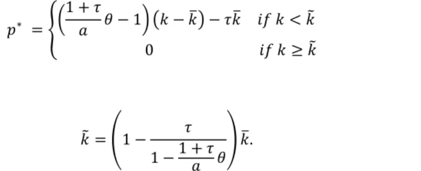
Note that 𝑒∗ in Eq. (18) is the marginal cost, 𝑀𝐶(𝑝, 𝑘). If 𝑘 < (1 − 𝜏)𝑘̅, there exists a unique
11
𝑝∗such that 𝑀𝐵(𝑝∗) = 𝑀𝐶(𝑝∗, 𝑘). The second-order condition is satisfied. If 𝑘 ≥ (1 − 𝜏)𝑘̅, then 𝑀𝐵(𝑝∗) ≤ 𝑀𝐶(𝑝∗, 𝑘) for all 𝑝 ≥ 0, which implies 𝑝∗ = 0 . This relationship is depicted in Fig. 1.
Fig. 1 is here
Formally, using Eqs. (13), (18), and (19), we obtain
𝑝∗ = {(1 − 𝜏)𝑘̅ − 𝑘 𝑖𝑓 𝑘 < (1 − 𝜏)𝑘̅
0 𝑖𝑓 𝑘 ≥ (1 − 𝜏)𝑘̅ (20)
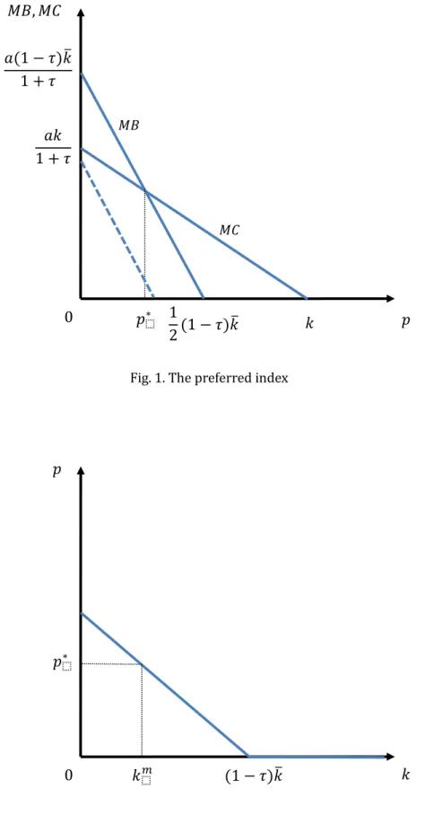
The relationship between wealth and the preferred index is shown in Fig. 2. Under the critical value(1 − 𝜏)𝑘̅ , this relationship is down sloping, while the preferred index is zero over the critical value.
Fig. 2 is here
The above argument can be summarized in the following proposition.
Proposition 1
Assume that 𝑘𝑚< (1 − 𝜏)𝑘̅. Then, the voting equilibrium is given by
𝑝𝑚= (1 − 𝜏)𝑘̅ − 𝑘𝑚. (21)
If 𝑘𝑚≥ (1 − 𝜏)𝑘̅, then the voting equilibrium is 𝑝𝑚= 0.
The intuition behind this proposition is as follows. If the median voter is a lower wealth household, the amount of child labor will be smaller (from Eq. (18)). As the wealth of median voter becomes greater, child labor increases, potentially resulting in a smaller share of the index.
Consequently, greater wealth (greater 𝑘𝑚) diminishes the share of index. Beyond a point, the median voter will choose 𝑝∗ = 0, that is, UCT programs.
Now we turn to the effects of the wealth inequality on child labor to consider the role of conditionality. For this purpose, we use the following index to measure wealth inequality,
𝑘̅ − 𝑘𝑚 𝑘̅ . From Eq. (21) the preferred index is rewritten as
𝑝𝑚= 𝑘̅ [𝑘̅ − 𝑘𝑚
𝑘̅ − 𝜏]. (22)
Whether conditionality in cash transfers is attached depends on the median of wealth, 𝑘𝑚, the average of wealth, 𝑘̅ , and tax rate, 𝜏 . Note that the first term on the right-hand side in the
12
square bracket of Eq. (22) represents the wealth inequality index. An increase in wealth inequality reduces child labor since the preferred index 𝑝∗ is decreasing in 𝑘 (from Eq. (20)).
This proposition suggests that CCTs tends to be preferred in the very unequal countries (Fiszbein and Schady, 2009). Since the key parameters that determine a condition is attached to cash transfers are the median of wealth, 𝑘𝑚, the average of wealth, 𝑘̅, and tax rate, 𝜏, we can make the cross-country estimates of the preferred index, 𝑝∗as explained in section 6.
The second term on the right-hand side in the square bracket of Eq. (22) is the tax effect.
From Eq. (18), we can see that the higher tax rate, the less child labor. Thus, as the redistribution effect through CCTs is small, the preferred index, 𝑝∗, is diminished.
5. Discussions
In this section, we extend our basic model to investigate whether CT programs may affect child labor supply across siblings. For this purpose, we change our basic model from Section 4 in two regards. First, to analyze the sibling effect on child labor and CT programs, we distinguish between farm work and domestic work such as caring for family members. Second, we introduce the heterogeneity of child labor (the age gap between siblings) into our basic model.
5.1 The sibling effect on child labor and CT programs
As pointed out by Patrinos and Psacharopoulos (1995, 1997), having a greater number of younger siblings implies more child labor. Thus, the number of younger siblings may affect child labor, and thereby the design of the CT programs. In this regard, we want to clarify this theory using our basic model based on the assumption that wealthier individual (more landholdings) have a greater number of children. In this subsection, we consider the different types of work performed by children. In particular, we distinguish the difference between farm work and domestic work such as caring for other children.
Older children’s time spent caring for younger siblings is assumed to 𝜃(𝑘). Since there are more younger siblings as the land is wider, we also assume 𝜃′ (𝑘) > 0. The more children there are in the household, the larger the household consumption expenditure. We also assume that the cost of childcare, 𝑐(𝑘), is not taxed (if it is taxed, the results are unchanged).
From the above assumption, we can rewrite the household budget constraint (2) as 𝑓(𝑘, 1 + 𝑒) + 𝑇̃ = (1 + 𝜏)𝑐 + 𝑐(𝑘).
Then, the utility function is modified by
𝑢 = 𝑢(𝑐, 𝑒; 𝑘) = 𝑐 − 𝜙(𝜃(𝑘) + 𝑒).
The household maximization problem is now given as
13 max 𝑒 𝑢 = 1
1 + 𝜏[𝑓(𝑘, 1 + 𝑒) + 𝑇 − 𝑝𝑒 − 𝑐(𝑘)] − 𝜙(𝜃(𝑘) + 𝑒) = 1
1 + 𝜏[𝑘(1 + 𝑒) + 𝑇 − 𝑝𝑒 − 𝑐(𝑘)] − 1
2𝑎(𝜃(𝑘) + 𝑒)2.
From the first-order conditions for utility maximization, we have child labor for household 𝑘 as 𝑒∗ =𝑎(𝑘 − 𝑝)
1 + 𝜏 − 𝜃(𝑘). (23)
Comparing this with Eq. (18), we can see that Eq. (23) reduces only the amount of 𝜃(𝑘).
The household’s consumption is rewritten as 𝑐 = 1
1 + 𝜏[𝑘(1 + 𝑒∗) + 𝑇 − 𝑝𝑒∗ − 𝑐(𝑘)].
The government budget constraint is 𝜏 ∫ 𝑐
𝐾
𝑑𝐹(𝑘) = ∫ (𝑇 − 𝑝𝑒∗)
𝐾
𝑑𝐹(𝑘), which gives
𝑇 = 𝜏 ∫ 𝑘(1 + 𝑒∗) − 𝑐(𝑘))𝑑𝐹(𝑘)
𝐾
+ 𝑝 ∫ 𝑒∗
𝐾
𝑑𝐹(𝑘) = 𝑇(𝑝, 𝜏). (24) Thus, the indirect utility function is given as
𝑢∗ = 1
1 + 𝜏[𝑘(1 + 𝑒∗) + 𝑇(𝑝, 𝜏) − 𝑝𝑒∗ − 𝑐(𝑘)] − 1
2𝑎(𝜃(𝑘) + 𝑒∗)2. Differentiating 𝑢∗ with respect to 𝑝, we obtain
𝜕𝑢∗
𝜕𝑝 = 1
1 + 𝜏[𝑘𝑒∗ + 𝑇𝑝 − 𝑒∗ − 𝑝𝑒𝑝∗] −1
𝑎(𝜃(𝑘) + 𝑒∗)𝑒𝑝∗ = 1
1 + 𝜏[𝑇𝑝 − 𝑒∗].
Thus, the preferred index for household 𝑘 is satisfied
𝑇𝑝 − 𝑒∗ = 0. (25)
From Eqs. (23) and (24), we obtain 𝑇𝑝 = 𝜏 ∫ 𝑘𝑒𝑝∗𝑑𝐹(𝑘)
𝐾
+ ∫ 𝑒∗
𝐾
𝑑𝐹(𝑘) + 𝑝 ∫ 𝑒𝑝∗ 𝐾
𝑑𝐹(𝑘)
= 𝑎
1 + 𝜏[(1 − 𝜏)𝑘̅ − 2𝑝] − ∫ 𝜃(𝑘)
𝐾
𝑑𝐹(𝑘).
Therefore, Eqs. (23) and (25) yields 𝑝∗ = (1 − 𝜏)𝑘̅ − 𝑘 +1 + 𝜏
𝑎 [𝜃(𝑘) − ∫ 𝜃(𝑘)
𝐾
𝑑𝐹(𝑘)]. (26)
14
When the caring time is constant, 𝜃(𝑘) = 𝜃̅, equation (26) is equal to be 𝑝∗ = (1 − 𝜏)𝑘̅ − 𝑘, which is the same as the first line of Eq. (20) in our basic model.
Note that if the cost of childcare depends on the number of children (the amount of land), the preferred index is different from the one in our basic model. To clarify this point, we assume 𝜃(𝑘) = 𝜃𝑘. In this specification, 𝜃 can be interpreted as additional time spent on domestic work. This means that when 𝜃 is higher, older children spent more time caring for younger siblings.
From Eq. (26), we obtain
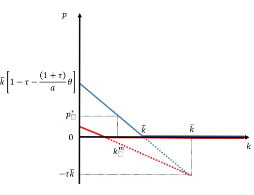
𝑝∗ = (1 − 𝜏)𝑘̅ − 𝑘 +1 + 𝜏
𝑎 𝜃(𝑘 − 𝑘̅) = (1 + 𝜏
𝑎 𝜃 − 1) (𝑘 − 𝑘̅) − 𝜏𝑘̅. (27)
When the horizontal axis indicates wealth (landholdings), 𝑘, and the vertical axis indicates the preferred index, 𝑝∗, equation Eq. (27) can be depicted on the (𝑘, 𝑝∗ ) plane. This relationship is depicted in Fig. 3.
Fig. 3 is here
Eq. (27) is a downward sloping straight line with slope (1 + 𝜏)𝜃/𝑎 − 1 and always passes the point (𝑘̅, −𝜏𝑘̅). Considering 𝑝∗ ≥ 0, we have
𝑝∗ = {(1 + 𝜏
𝑎 𝜃 − 1) (𝑘 − 𝑘̅) − 𝜏𝑘̅ 𝑖𝑓 𝑘 < 𝑘̃
0 𝑖𝑓 𝑘 ≥ 𝑘̃
(28)
where
𝑘̃ = (1 − 𝜏 1 −1 + 𝜏
𝑎 𝜃
) 𝑘̅. (29)
If 𝜃 = 0, then 𝑘̃ = (1 − 𝜏)𝑘̅, and Eq. (28) is the same as the first line of Eq. (20). Assuming that 𝜃 increases from zero, the slope of Eq. (28) declines past the point (𝑘̅, −𝜏𝑘̅). Thus, for the household 𝑘 < 𝑘̃,
𝜕𝑝∗
𝜕𝜃 < 0.
is satisfied. This result means that the more younger siblings in the household, the smaller the index supported for a landless household, that is, landless household tends to prefer to UCT programs.
15 Fig. 4 is here
The intuition behind this result is as follows. Like our basic model presented in Section2, the marginal benefit (MB) of increasing the index share, 𝑝, is 𝑇𝑝 and the marginal cost (MC) is 𝑒∗. From Eq. (23), we can see that the MC declines by the amount of 𝜃𝑘 when 𝜃(𝑘) = 𝜃𝑘.
On the other hand, the MB also declines by the amount of 𝜃𝑘̅ . Note that, for the landless households, 𝜃𝑘 < 𝜃𝑘̅ is satisfied. In other words, the negative effect of reducing the MB dominated the positive effect of a decrease in the MC (see, Fig. 4). Thus, a smaller share of the index is supported by landless household.
In contrast, land-rich households have incentives to support a larger share of the index due to the larger positive effect from the decrease in MC. However, as it binds 𝑝∗ ≥ 0 and their opinions are not reflected through their voting decision, their vote does not affect the voting equilibrium. Therefore, we have the following proposition,
Proposition 2.
Assume that 𝜃(𝑘) = 𝜃𝑘. If 𝑘𝑚 < 𝑘̃, then the voting equilibrium is given by 𝑝𝑚= (1 + 𝜏
𝑎 𝜃 − 1) (𝑘𝑚− 𝑘̅) − 𝜏𝑘̅. (30)
If 𝑘𝑚> 𝑘̃, the voting equilibrium is 𝑝𝑚= 0.
Now, we focus on the effects on the equilibrium amount of child labor. Making use of Eqs. (25) and (30), we can rewrite Eq. (23) as
𝑒∗(𝑘, 𝜏, 𝜃) =𝑎[𝑘 − 𝑝𝑚(𝑘, 𝜏, 𝜃)]
1 + 𝜏 − 𝜃𝑘. (31)
The effect on the equilibrium amount of child labor of additional time spent on domestic work can be interpreted as follows. From the first term on the right-hand side of Eq. (31), we can see that an increase in 𝜃 leads to more work on the family farm thorough a decrease in the preferred index. Since the government imposes a penalty only for child farm work, when this penalty is small, poor parents may have their children work more on the family farm. On the other hand, from the second term on the right-hand side of Eq. (31), an increase in 𝜃 declines the equilibrium amount of child labor. Then, the overall effect on the equilibrium amount child labor is ambiguous, depending on the relative magnitudes of these two effects. The equilibrium amount of child labor can be further rewritten as
𝑒∗(𝑘, 𝜏, 𝜃) = 𝑎
1 + 𝜏{𝑘 − (1 + 𝜏
𝑎 𝜃 − 1) (𝑘𝑚− 𝑘̅) − 𝜏𝑘̅} − 𝜃𝑘. (32) From Eq. (32), we can drive the following corollary:
16 Corollary 1.
(i) when 𝑘 < 𝑘̅ − 𝑘𝑚, 𝜕𝑒∗⁄𝜕𝜃 > 0. (ii) when 𝑘 > 𝑘̅ − 𝑘𝑚, 𝜕𝑒∗⁄𝜕𝜃 < 0.
The intuition behind this corollary can be explained as follows. For land-poor households, when older siblings spend more time engaged in domestic work, the majority tend to support UCT programs (𝜕𝑝∗⁄𝜕𝜃 < 0). As a result, for poor countries, the introduction of CT programs may provide an incentive for land-poor households to have their children work more on the family farm. This theoretical result is consistent with empirical evidences of Edmonds (2006, p.817, p.819), who observed both males and females work more in the presence of younger male siblings. As household size increases, the extra work associated with being an older girl increases significantly. Most of this additional work for girls comes from spending additional time in domestic activities such as childminding, cooking, and cleaning. This corollary also suggests that there is no substitution within the household of younger for older siblings in domestic work, as pointed out by Dammert (2010), who found the relevance of domestic work and gender differentials in children’s allocation of time in Nicaragua and Guatemala.
In contrast, as they have greater wealth, more time spent on domestic work leads to less farm work, which is substitutable for domestic work. In this case, the negative domestic child labor effect exceeds the positive farm child labor effects.
5.2 Heterogenous child labor
We next introduce the heterogeneity of labor efficiency into our basic model. We assume that each parent has two children who have different levels child labor efficiency; one child has a higher marginal product in household production than the other. This assumption of comparative advantage in household production is consistent with findings by Edmonds (2007), who argued that working older siblings may provide additional labor services to the household, which lowers the productivity of younger siblings. In this setting we show that the lower the labor efficiency of one child, the lower the share of preferred index. Therefore, households with lower productivity of younger siblings tend to support the UCT programs.
The household budget constraint is rewritten as
𝑓(𝑘, 1 + 𝑒1 + 𝜀𝑒2) + 𝑇̃ = (1 + 𝜏)𝑐 + 𝑐(𝑘),
where 𝑒𝑖 is the working time of child 𝑖 (𝑖 = 1,2); the labor efficiency of child 2 is 𝜀 ≤ 1. This assumption means that we can interpret one child as having a comparative advantage in household production compared to the other. As pointed out by Edmonds (2006), the existence of household production implies that the age and sex composition of siblings affects a
17
child’s labor supply. 𝑐(𝑘) is the cost of childcare (not taxed).
The utility function is now
𝑢 = 𝑢(𝑐, 𝑒) = 𝑐 − 𝜙(𝑒1 ) − 𝜙(𝑒2).
We assume that parents consider leisure as a luxury good for each child and that they know the labor efficiency of each child.
Instead of the specification in Eq. (3), the CT program is modified as 𝑇̃ = 𝑇 − 𝑝(𝑒1 + 𝑒2).
The household maximization problem is max𝑒 𝑢 = 1
1 + 𝜏[𝑓(𝑘, 1 + 𝑒1 + 𝜀𝑒2) + 𝑇 − 𝑝(𝑒1 + 𝑒2) − 𝑐(𝑘)] − 𝜙(𝑒1 ) − 𝜙(𝑒2) = 1
1 + 𝜏[𝑘(1 + 𝑒1 + 𝜀𝑒2) + 𝑇 − 𝑝(𝑒1 + 𝑒2) − 𝑐(𝑘)] − 1
2𝑎(𝑒1)2 − 1 2𝑎(𝑒2 )2 The first-order conditions require
𝜕𝑢
𝜕𝑒1 =𝑘 − 𝑝 1 + 𝜏−𝑒1
𝑎 = 0,
𝜕𝑢
𝜕𝑒2 =𝑘𝜀 − 𝑝 1 + 𝜏 −𝑒2
𝑎 = 0.
which gives child labor as
𝑒1∗=𝑎(𝑘 − 𝑝)
1 + 𝜏 , (33a)
𝑒2∗=𝑎(𝑘𝜀 − 𝑝)
1 + 𝜏 . (33b)
The household consumption is given by 𝑐 = 1
1 + 𝜏[𝑘(1 + 𝑒1∗+ 𝜀𝑒2∗) + 𝑇 − 𝑝(𝑒1∗+ 𝑒2∗) − 𝑐(𝑘)].
The government budget constraint is 𝜏 ∫ 𝑐
𝐾
𝑑𝐹(𝑘) = ∫ 𝑇̃
𝐾
𝑑𝐹(𝑘).
Substituting household consumption and the CT program into the government budget constraint, we obtain the uniform transfer as a function of (𝑝, 𝜏),
𝑇 = 𝜏 ∫ [𝑘(1 + 𝑒1∗+ 𝜀𝑒2∗) − 𝑐(𝑘)]𝑑𝐹(𝑘)
𝐾
+ 𝑝 ∫ (𝑒1∗+ 𝑒2∗)
𝐾
𝑑𝐹(𝑘) = 𝑇(𝑝, 𝜏).
Then, the indirect utility function of household 𝑘 is rewritten as 𝑢∗ = 1
1 + 𝜏[𝑘(1 + 𝑒1∗+ 𝜀𝑒2∗) + 𝑇(𝑝, 𝜏) − 𝑝(𝑒1∗+ 𝑒2∗) − 𝑐(𝑘)] − 1
2𝑎(𝑒1 )2 − 1
2𝑎(𝑒2 )2. Differentiating 𝑢∗ with respect to 𝑝, and using the first-order conditions, we obtain
18
𝜕𝑢∗
𝜕𝑝 = 1
1 + 𝜏[𝑇𝑝 (𝑝, 𝜏) − (𝑒1∗+ 𝑒2∗)].
Therefore, the preferred index for household 𝑘, denoted by 𝑝∗ = 𝑝(𝑝, 𝜏) is given by 𝑇𝑝 (𝑝, 𝜏) = 𝑒1∗(𝑘, 𝑝∗ , 𝜏) + 𝑒2∗(𝑘, 𝑝∗, 𝜏).
The marginal benefit is now
𝑇𝑝 = 𝜏 ∫ 𝑘(𝑒1𝑝∗ + 𝑒2𝑝∗ )𝑑𝐹(𝑘)
𝐾
+ ∫ (𝑒1∗+ 𝑒2∗)
𝐾
𝑑𝐹(𝑘) + 𝑝 ∫ (𝑒1𝑝∗ + 𝑒2𝑝∗ )
𝐾
𝑑𝐹(𝑘)
= 𝜏 ∫ 𝑘 [(− 𝑎
1 + 𝜏) + 𝜀 (− 𝑎
1 + 𝜏)] 𝑑𝐹(𝑘)
𝐾
1 1 + 𝜏 + ∫ [(𝑎(𝑘 − 𝑝)
1 + 𝜏 ) + (𝑎(𝑘𝜀 − 𝑝) 1 + 𝜏 )]
𝐾
𝑑𝐹(𝑘)
+𝑝 ∫ 𝑘 [(− 𝑎
1 + 𝜏) + 𝜀 (− 𝑎 1 + 𝜏)]
𝐾
𝑑𝐹(𝑘)
= 𝑎
1 + 𝜏[(1 + 𝜀)(1 − 𝜏)𝑘̅ − 4𝑝] = 𝑀𝐵(𝑝, 𝜀).
The marginal cost is
𝑒1∗+ 𝑒2∗= 𝑎
1 + 𝜏[(1 + 𝜀)𝑘 − 2𝑝] = 𝑀𝐶(𝑝, 𝜀).
When the horizontal axis indicates the preferred index, 𝑝∗, and the vertical axis indicates the marginal benefit and the marginal cost, if 𝑘 < (1 − 𝜏)𝑘̅ is satisfied, there is an intersection between 𝑀𝐵(𝑝, 𝜀) and 𝑀𝐶(𝑝, 𝜀) . To the left of intersection point, 𝑀𝐵 > 𝑀𝐶 is satisfied, and to the right of intersection point, 𝑀𝐵 < 𝑀𝐶 is satisfied. Then, household utility is maximized at the intersection point, 𝑝∗. Solving 𝑀𝐵(𝑝, 𝜀) = 𝑀𝐶(𝑝, 𝜀), we obtain
𝑝∗ =1
2(1 + 𝜀)[(1 − 𝜏)𝑘̅ − 𝑘]. (34)
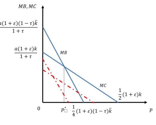
If 𝑘 ≥ (1 − 𝜏)𝑘̅, it satisfied 𝑀𝐵(𝑝, 𝜀) ≥ 𝑀𝐶(𝑝, 𝜀) for all 𝑝, then 𝑝∗ = 0.This relationship is depicted in Fig. 5.
Fig. 5 is here
When the siblings have the same labor efficiency (𝜀 = 1), Eq. (34) is equal to the first line of Eq. (20) in our basic model. When the siblings have the different labor efficiency (𝜀 < 1), the preferred index for household 𝑘 is lower. This reason is as follows. A decrease in labor efficiency induces the marginal benefit to shift downward by 𝑎(1 − 𝜏)𝑘̅ (1 + 𝜏)⁄ . Thus, the intersection point shifts to the left. On the other hand, the marginal cost shifts downward by 𝑎𝑘 (1 + 𝜏)⁄ . Thus, the intersection point shifts to the right. Overall, whether the intersection
19
point shifts to the right or left depends on the slope of the marginal benefit and marginal cost.
In the light of absolute value, the slope of the marginal benefit is greater than that of the marginal cost. Hence, the intersection point shifts to the left because the negative effect of the reduction in marginal benefit dominates the positive effect of the reduction of marginal cost (see, Fig. 5).
Summarizing the above, we have the following proposition:
Proposition 3.
Assume that 𝑘𝑚≤ (1 − 𝜏)𝑘̅. Then, the voting equilibrium is given by 𝑝𝑚=1
2(1 + 𝜀)[(1 − 𝜏)𝑘̅ − 𝑘𝑚]. (35)
𝑝𝑚 is positively related to the sibling’s labor productivity, 𝜀. If 𝑘𝑚> (1 − 𝜏)𝑘̅, then 𝑝𝑚= 0.
Now we turn to the effects on the equilibrium amount of child labor. Substituting Eqs. (33a) and (33b) into Eq. (35), the equilibrium amount of child labor among siblings is rewritten as
𝑒1∗(𝑘𝑚, 𝜏, 𝜀) = 𝑎
1 + 𝜏{𝑘 −1
2(1 + 𝜀)[(1 − 𝜏)𝑘̅ − 𝑘𝑚]}, (36a) 𝑒2∗(𝑘𝑚, 𝜏, 𝜀) = 𝑎
1 + 𝜏{𝜀𝑘 −1
2(1 + 𝜀)[(1 − 𝜏)𝑘̅ − 𝑘𝑚]}. (36b) From Eq. (36a), we have the following corollary:
Corollary 2.
A narrowing age gap leads to a reduction in the amount of older children’s work.
In this subsection, the sibling’s labor productivity, 𝜀 , is of central interest. 𝜀 can also be interpreted as the age gap between siblings, and an increase in 𝜀 means that the age gap narrows. Note that, from Eq. (36a), when the age gap becomes smaller, the amount of older children’s child labor is reduced through the effects of an increase in the share of the index.
This theoretical result is consistent with empirical evidences of Edmonds (2006, p.816), who found both older males and older females have to work less as the age gap decreases.
In contrast, the effect of the narrowed age gap on child labor of the younger sibling is ambiguous. The amount of total child labor is
𝑒1∗+ 𝑒2∗= 𝑎
1 + 𝜏{(1 + 𝜀)𝑘 − (1 + 𝜀)[(1 − 𝜏)𝑘̅ − 𝑘𝑚]}
=𝑎(1 + 𝜀)
1 + 𝜏 {𝑘 − [(1 − 𝜏)𝑘̅ − 𝑘𝑚]}. (37)
From Eqs. (36b) and (37), we can drive the following corollary:
20 Corollary 3.
(i) when 𝑘 <1
2[(1 − 𝜏)𝑘̅ − 𝑘𝑚], 𝜕𝑒2∗⁄∂𝜀 < 0 and 𝜕(𝑒1∗+𝑒2∗) ∂𝜀 < 0⁄
(ii) when 1
2[(1 − 𝜏)𝑘̅ − 𝑘𝑚] < 𝑘 < [(1 − 𝜏)𝑘̅ − 𝑘𝑚], 𝜕𝑒2∗⁄∂𝜀 > 0 and 𝜕(𝑒1∗+𝑒2∗) ∂𝜀 < 0⁄ . (iii) when 𝑘 > [(1 − 𝜏)𝑘̅ − 𝑘𝑚], 𝜕𝑒2∗⁄∂𝜀 > 0 and 𝜕(𝑒1∗+𝑒2∗) ∂𝜀 > 0⁄
The intuition behind this corollary can be explained as follows. When a household’s wealth is smaller enough, a narrowed age gap leads to support CCT programs by the majority (from Eq.
(35)). From Eq. (36b), we can see that the effect of CT programs dominates the wealth effect.
As a result, for poor countries, the introduction of CT programs may decrease both the total amount of child labor and the labor of the younger sibling. This result is consistent with findings by Edmonds (2006, p.819), who demonstrated that for small age gaps, a subsequent female sibling is associated with less additional work for both boys and girls in both market and domestic work. Another finding is a program in Cambodia by Ferreira et al., (2017), who argued that CCTs have a negative displacement effect on siblings.13 They also pointed out that this ambiguity arises from the interaction of a positive income effect with a negative displacement effect. In our model, we could explain this result for the wealth heterogeneity (landholdings).
As the household’s wealth is larger, a decrease in the age gap induces an increase in the amount of younger children’s child labor.
6. Calibrations
So far we have focused on the design of CT programs (conditional or unconditional), which is decided through a political process. As pointed out in the Introduction, Gaarder (2014), among others argued that while most CT programs in Latin America are conditional, the majority of them in sub-Saharan Africa are unconditional. Using our model, we try to explain why these distinctions occur in developing and transition economies. From equation (22), we can find the key parameters that determine whether a condition is attached to cash transfers are the median of wealth, 𝑘𝑚 , the average of wealth, 𝑘̅ and tax rate, 𝜏 .14 Then we first obtain the
13 So far, as Fiszbein and Schady (2009, p.116) pointed out, CT programs could potentially have positive or negative spillovers for other siblings: positive if the income effect reduces child work for all children; negative if parents compensate for the reduction in the work of one child by increasing the work of other sibling in many developing countries. Recently, Ferreira et al., (2017) added to the third effect as a negative displacement effect that CT programs might lead parents to reallocate child work away from the recipient and to other children in the household.
14 In this section, we assume away the tax rate, 𝜏, although we can use the tax data such as the 2018 World Development Indicators (WDI) database of the World Bank, because many countries
21
cross-country estimates of the preferred index, 𝑝𝑚. Our result confirms that a number of countries with a greater wealth inequality adopt conditional cash transfers in developing and transition economies.
The median and mean wealth data are both obtained from Davies et al., (2017), who provided the estimates of the global distribution of wealth for the period 2000-2014.15 The Credit Suisse Research Institute (2010, p.95) argued that when we look at the relative importance of financial versus non-financial assets in the average household portfolio, especially, in developing countries, it is not unusual for 80% or more of total assets to be held in the form of non-financial assets, including farms, and small business assets. This pattern is also associated with the relative under-development of financial institutions in many lower income countries. The countries that introduced CCTs are from Fiszbein and Schady (2009) and World Bank (2015) and, the other countries, including those adopting UCTs, are from Garcia et al., (2011) and World Bank (2015). From those countries and the data obtained from Davies et al., (2017), we focus on those with a population of more than one million, and a mean wealth of less than 30,000 USD. There are 52 countries with CCTs (see Table 1) and 36 other countries, including those adopting UCTs (see Table 2).
Table 1. and Table 2. are Here.
Fig. 6 plots the inequality index among CCTs and other countries, including those adopting UCTs, against the mean wealth of less than 30,000 USD used in Table 1 and Table 2. From observing that the differences between CCTs and other countries appears through the inequality index using both the median and mean wealth, we can confirm that a number of countries with greater wealth inequality tend to adopt conditional cash transfers in developing and transition economies.
Fig. 6. is Here.
In this section, we explore whether there is any significant difference between CCTs and other countries (including those adopting UCTs). Between-group comparisons (i.e., CCTs and other countries) were assessed using independent t-tests.
that implement both CCTs and UCTs are supported and promoted by multilateral banks, such as the World Bank and the Inter-American Development Bank. In the African case, international donors such as DFID and UNICEF also have played a more central role (Gaarder, 2014).
15 Davies et al., (2017) define the distribution of net worth within and across nations as the market value of financial assets plus non-financial assets (principally housing and land) less debts. Private pension wealth is included, but public pensions are not.
22 Table 3. is Here.
Table 3 summarizes the results of independent t-tests used to compare the data. An independent t-test revealed a significant difference between groups (𝑝 = 0.00060916). This result shows that there is a different in the inequality index between the two groups.
7. Concluding Remarks
This paper examines the role of conditionality in the choice between CCTs and UCTs for CT programs to eliminate child labor. We consider an overlapping generations model à la Basu et al., (2010), who demonstrated the inverted-U relationship between wealth (especially landholding) and child labor. We show that when wealth inequality is high, CCTs tend to be supported by median voters, and child labor is reduced. In contrast, UCTs tend to have political support when there is little wealth inequality across individuals, but child labor prevails. Our cross-country estimation confirmed that a number of countries with greater wealth inequality tend to adopt CCTs in developing and transition economies. We also examine whether attaching condition to cash transfers generates sibling differences in child labor.
We have not considered the inequality-growth relationship in the choice between CCTs and UCTs for CT programs. As pointed out by Barrientos and DeJong (2006), one of the main aims of the CT programs is to enhance investment in human capital. We also assume away the role of education and health component to focus on the “wealth paradox”, as noted in Basu et al., (2010). Many studies on CCTs shed light on the specific behavior of the beneficiary households such as school enrolment and attendance of children, regular use of primary health care by mothers and infants. These and other possible improvement in this paper are subjects for future research.
23 References
Akresh, R., De Walque, D. and Kazianga, H., 2013. Cash transfers and child schooling: Evidence from a randomized evaluation of the role of conditionality. World Bank Policy Research Working Paper, 6340.
Alvi, E. and Dendir, S., 2011. Sibling differences in school attendance and child labour in Ethiopia.
Oxford Development Studies, vol. 39(3), pp. 285-313.
Attanasio, O. P., Meghir, C. and Santiago, A., 2012. Education choices in Mexico: Using a structural model and a randomized experiment to evaluate Progresa. The Review of Economic Studies, vol. 79(1), pp. 37-66.
Baird, S., Ferreira, F. H., Özler, B. and Woolcock, M., 2014. Conditional, unconditional and everything in between: A systematic review of the effects of cash transfer programmes on schooling outcomes. Journal of Development Effectiveness, vol. 6(1), pp. 1-43.
Baird, S., McIntosh, C. and Özler, B., 2011. Cash or condition? Evidence from a cash transfer experiment. The Quarterly Journal of Economics, vol. 126, pp. 1709-1753.
Bar, T. and Basu, K., 2009. Children, education, labor, and land: in the long run and short run.
Journal of the European Economic Association, vol. 7(2-3), pp. 487-497.
Barrera-Osorio, F., Bertrand, M., Linden, L. L. and Perez-Calle, F., 2011. Improving the design of conditional transfer programs: Evidence from a randomized education experiment in Colombia. American Economic Journal: Applied Economics, vol. 3(2), pp. 167-95.
Barrientos, A. and DeJong, J., 2006. Reducing child poverty with cash transfers: A sure thing?
Development Policy Review, vol. 24(5), pp. 537-552.
Basu, K., Das, S. and Dutta, B., 2010. Child labor and household wealth: Theory and empirical evidence of an inverted-U. Journal of Development Economics vol. 91, pp. 8-14.
Basu, K. and Tzannatos, Z., 2003. The global child labor problem: What do we know and what can we do? The World Bank Economic Review, vol. 17(2), pp. 147-173.
Bearse, P., Glomm, G., and Ravikumar, B., 2000. On the political economy of means-tested education vouchers. European Economic Review, 44(4-6), 904-915.
Behrman, J. R., Sengupta, P. and Todd, P. 2005., Progressing through PROGRESA: An impact assessment of a school subsidy experiment in rural Mexico. Economic Development and Cultural Change, vol. 54(1), pp. 237-275.
Behrman, J. R. and Skoufias, E. 2006., Mitigating myths about policy effectiveness: Evaluation of Mexico’s antipoverty and human resource investment program. The Annals of the American Academy of Political and Social Science, vol. 606(1), pp. 244-275.
Bhalotra, S. and Heady, C., 2003. Child farm labor: The wealth paradox. The World Bank Economic Review, vol. 17(2), pp. 197-227.
Bourguignon, F., Ferreira, F. H. and Leite, P. G., 2003. Conditional cash transfers, schooling, and
24
child labor: Micro-simulating Brazil's Bolsa Escola program. The World Bank Economic Review, vol. 17(2), pp. 229-254.
Borck, R., 2007. On the choice of public pensions when income and life expectancy are correlated.
Journal of Public Economic Theory, vol. 9, pp. 711-725.
Cardoso, E. and Souza, A. P., 2004. The impact of cash transfers on child labor and school attendance in Brazil. Vanderbilt University Department of Economics Working Papers 0407, Vanderbilt University Department of Economics.
Casamatta, G., Cremer, H. and Pestieau, P., 2000. Political sustainability and the design of social insurance. Scandinavian Journal of Economics, vol. 75, pp. 341-364.
Cigno, A., 2008. Is there a social security tax wedge? Labour Economics, vol. 15, pp. 68-77.
Cockburn, J. and Dostie, B., 2007. Child work and schooling: The role of household asset profiles and poverty in rural Ethiopia. Journal of African Economies, vol. 16(4), pp. 519-563.
Conde-Ruiz, J.I. and Profeta, P., 2007. The redistributive design of social security systems.
Economic Journal, vol. 117, pp. 686-712.
Covarrubias, K., Davis, B. and Winters, P., 2012. From protection to production: Productive impacts of the Malawi social cash transfer scheme. Journal of Development Effectiveness, vol.
4(1), pp. 50-77.
Credit Suisse Research Institute., 2010. Global Wealth Report, Zurich: Credit Suisse Research Institute.
Cremer, H., De Donder, P., Maldonado. D. and Pestieau, P., 2007. Voting over type and generosity of a pension system when some individuals are myopic. Journal of Public Economics, vol. 91, pp. 2041-2061.
Dammert, A. C., 2010. Siblings, child labor, and schooling in Nicaragua and Guatemala. Journal of Population Economics, vol. 23(1), pp. 199-224.
Davies, J. B., Lluberas, R. and Shorrocks, A. F., 2017. Estimating the level and distribution of global wealth, 2000-2014. Review of Income and Wealth, vol. 63(4), pp. 731-759.
Davis, B., Gaarder, M., Handa, S. and Yablonski, J., 2012. Evaluating the impact of cash transfer programmes in sub-Saharan Africa: An introduction to the special issue. Journal of Development Effectiveness, vol. 4(1), pp. 1-8.
De Haan, M., Plug, E. and Rosero, J., 2014. Birth order and human capital development evidence from Ecuador. Journal of Human Resources, vol. 49(2), pp. 359-392.
De Hoop, J. and Rosati, F. C., 2014. Cash transfers and child labor. The World Bank Research Observer, vol. 29(2), pp. 202-234.
De Janvry, A. and Sadoulet, E., 2006. Making conditional cash transfer programs more efficient:
Designing for maximum effect of the conditionality. The World Bank Economic Review, vol.
20(1), pp. 1-29.