Submitted to the Department of Earth and Planetary Sciences

(1)

九州大学学術情報リポジトリ

Kyushu University Institutional Repository

大気ブロッキングの持続メカニズムについて

山崎, 哲

九州大学大学院理学府

https://doi.org/10.15017/21709

出版情報：Kyushu University, 2011, 博士（理学）, 課程博士バージョン：

権利関係：

(2)

The Maintenance Mechanism of Atmospheric Blocking

by

Akira Yamazaki

Submitted to the Department of Earth and Planetary Sciences

in Partial Fulfillment of the Requirements for the Degree of

Doctor of Science at

Kyushu University

February 2012

(3)

Abstract

A new eddy-feedback mechanism, the Selective Absorption Mechanism (SAM), to explain the block maintenance is proposed. In this mechanism which is based on the vortex-vortex interaction, that is, the interaction mechanism of a blocking anticyclone and synoptic eddies with the same polarity, a blocking anticyclone actively and selectively absorbs synoptic anticyclones. The blocking anticyclone thus supplied with low potential vorticity can last for a long time against dissipation.

The SAM is verified by two main analyses. The first is to examine ten real cases of blocking using trajectory analysis. Trajectories are calculated by tracing parcels originating from synoptic anticyclones and cyclones upstream of blocking. Parcels starting from anticyclones are attracted and absorbed by the blocking anticyclone, whereas parcels from cyclones are repelled by it and attracted by the blocking cyclone if it exists.

The second analysis is to conduct numerical experiments using the nonlinear equivalent- barotropic potential vorticity equation with some diﬀerent conditions, which are in shape and amplitude of blocking and in variabilities (displacement and strength) of stormtracks.

These experiments indicate that the SAM eﬀectively works to maintain the blocking with- out depending on these conditions.

These results show that the SAM is the general maintenance mechanism of blocking.

Next, some possible applications of the SAM are mentioned. First, the SAM is applied to a quantitative estimation of the interaction between a blocking anticyclone and synoptic anticyclones in real situations. The eﬀect of the forcing by the interaction between the blocking anticyclone and synoptic ones is estimated. The response to this forcing in a barotropic model well explains the pattern and amplitude of real blocking. Thus, the interaction with synoptic anticyclones plays an important role in the block maintenance.

(4)

Second, the SAM is adapted to a block in summer when the activity of synoptic eddies is thought to be the minimum during a year. However, it is found that the variability of potential vorticity is climatologically the maximum in summer, which implies that the SAM can also be adopted to summer blocking. Then, a case study for the 2010 summertime blocking is performed for investigating whether the SAM actually contributes to the maintenance of this blocking. Through the trajectory analysis, an analysis of ensemble forecast data, and a barotropic model experiment, the maintenance of this summertime blocking is found to be also largely contributed by the selective absorption of synoptic anticyclones. Thus, even in summer, the SAM can be essential for the maintenance of blocking.

(5)

Chapter 1 Introduction

1.1 A review

Atmospheric blocking is a quasi-stationary pattern characterized by a pronounced me- andering toward high latitudes of the westerly jetstream in middle latitudes or by a split of it into two distinctly separated currents, lasting about one week or more. The pattern is accompanied by a large-amplitude anticyclone with equivalent-barotropic structure on its poleward side. The anticyclone shows anΩ-shape in a synoptic field. Another type, a dipole structure with a cyclone on the equatorial side, also sometimes appears. We call the former an Ω-type block and the latter a dipole-type one. The anticyclone/cyclone is called a blocking anticyclone/cyclone. These blocks literally ‘block’ synoptic eddies drifting from upstream.

Since an anomalous pattern of blocking persists for a long time, blocks are related to various weather extremes, hence causing various disasters. A typical example is the record-breaking summer of 2010. A blocking anomaly persisting from July through mid- August over western Russia caused an extreme heat wave in western Russia and flooding in Pakistan and northwestern India (Dole et al. 2011; Hong et al. 2011).

Blocking is also a key phenomenon in medium-range weather forecasting, because it is not enough accurately reproduced in numerical prediction even in the present day when its techniques have been fairly developed (Kimoto et al. 1992; Pelly and Hoskins 2003a).

Moreover, since occurrence and persistence of blocks largely aﬀect climate in one season, it is important that climate models can reproduce blocking well. It is, however, reported

(8)

that this reproduction is not good enough (e.g., D’Andrea et al. 1998; Matsueda et al.

2009; Scaife et al. 2010). Thus, a wide spectrum of interest is directed toward blocking, as well as scientific interest.

Scientific interest is, of course, very high. There have been numerous studies about blocking, since Garriott first discovered blocking in 1904 (Rex 1950). The central issue among many research aspects of blocking may be its mechanism. However, it is still unclear, although over 100 years have already passed since its discovery. There can be no doubt that the understanding of the blocking mechanism is a key to improve the forecast of blocking, and thereby to prevent or lessen disasters associated with blocking.

In order to clarify the mechanism of blocking, we think it is important to explicitly distinguish between the two mechanisms, formation and maintenance (also see Mullen 1987); blocking has obviously diﬀerent time scales between its formation or onset and maintenance. The former scale is about 1 to 2 days, while the latter one is longer than the typical time scale of synoptic eddies. This implies that even instantaneous happenings can cause the onset, whereas continuous or periodic source against dissipation is needed for the maintenance. Some theories for the blocking mechanism have been proposed; for instance, theories of local nonlinear resonance (Pierrehumbert and Malguzzi 1984) and local Rossby wave breaking (Nakamura, H. 1994; Naoe and Matsuda 2002). However, these theories would be appropriate for the formation of blocking but not the maintenance, since resonance alone cannot guarantee the maintenance (no source), and Rossby wave breaking does not always occur in blocking regions (no continuous source). Thus these theories would be diﬃcult to be applied to the maintenance. Unlike these studies, the aim of this study is to explicitly propose a new maintenance mechanism of blocking.

Needless to say, the formation mechanism is important and must be elucidated, but it will be a future work.

One achievement of long-term studies on the maintenance mechanism of blocking is that synoptic eddies obstructed by blocking themselves enhance the blocking (e.g., Green 1977; Shutts 1983, 1986; Mullen 1986, 1987; Nakamura and Wallace 1993; Nakamura et al. 1997). Synoptic eddies are ubiquitous around blocking so that they can be contin-

(9)

uous source of the maintenance. Blocking also gives influence on synoptic eddies. Thus, synoptic eddies and blocking interact with each other. This interaction mechanism is called the eddy-feedback mechanism, which has been supported by many studies (some of them are cited above). We believe that there may be no other ways to maintain blocking necessarily and continuously but not accidentally. The maintenance mechanism proposed here is also on this framework.

1.2 The Eddy Straining Mechanism

This eddy-feedback mechanism is especially developed by Shutts (1983, hereafter S83), which is a milestone paper in the blocking theory. S83 proposed a well-known block maintenance mechanism, the Eddy Straining Mechanism (hereafter referred to as ESM), as a physical entity of the eddy-feedback. He demonstrated how eddies superimposed on uniform zonal westerly plus blocking flow behave and reinforce the blocking flow by numerical experiments with a linearized model. On the basis of his results, he suggested that synoptic eddies strained in the north-south direction by the blocking provide negative/positive vorticity forcing to the blocking anticyclone/cyclone; this vorticity forcing, i.e., the second-order induced flow maintains the blocking dipole structure against dissipation (Fig. 1.1). The eddy straining in the diﬄuent region of blocks has been found in many case studies, climatological ones, and numerical experiments (Hoskins et al. 1983;

Nakamura and Wallace 1993; Luo 2005; and many others). Then, the ESM has been widely popularized as a mainstream of the eddy-feedback mechanism. From a theoretical viewpoint, Nakamura, M. (1994) showed in his model evidence of the eddy straining in a region of jet splitting mimicking a blocking flow by using contour dynamics.

S83 also suggested that in the ESM the basic flow including the blocking flow deter- mines whether the eddy-feedback eﬀectively works or not; he showed that in the same linearized model but with diﬀerent basic flow, second-order flow patterns drastically change.

Thus, when basic flows satisfy proper conditions, then blocking can be spontaneously maintained due to the eddy-feedback.

S83 supported the ESM also by an analytical method. Supposing the existence of an

(10)

area bounded by an isopleth of eddy enstrophy just upstream of blocking, and integrating his eddy enstrophy equation related to the eddy straining over this area, he showed a balance between the terms of equatorward eddy vorticity flux and dissipation,

∫

Sens

ζ^′V^′· ∇( ¯ζ+ f)dS_ens= −E

∫

Sens

ζ^′²dS_ens, (1.1) where Sens denotes this area, ζ and f the relative and planetary vorticity, respectively, Vthe horizontal wind vector, E the Ekman friction coefficient, and ( ) and ( )^′ a time- averaged field and the deviation from it, respectively. This equation shows that the net equatorward eddy vorticity flux or its divergence/convergence in the north/south side just upstream of the blocking diffluent region counterbalances the dissipation (Section 2b of S83). He further showed that the net southward vorticity (or potential vorticity) flux corresponds to the eddy straining upstream of the jet-splitting. This eddy flux pattern is shown in two case studies by Illari (1984) and Shutts (1986) and in numerical simulations by S83, Haines and Marshall (1987), and Arai and Mukougawa (2002, hereafter referred to as AM02). More detailed and quantitative analyses for the eddy-feedback effect have been done in Mullen (1986, 1987), which investigated the budget of the eddy-feedback to composited blocks in both output data from a general circulation model and observational data. He concluded that eddy vorticity flux pattern obtained in both data is consistent with that predicted by the ESM and this eddy forcing mainly maintains the blocks in a quantitative sense. He also found that the eddy-feedback can counteract not only dissipation but also the advective effect by background westerlies (to advect blocks downstream).

1.3 Motivation of this thesis

Some recent studies, however, showed evidence that the ESM cannot fully explain the maintenance of blocking in real situations; the ESM has strong sensitivity to stormtrack conditions, though they considerably vary in real situations. AM02 demonstrated through their similar experiments to S83 that patterns of the second-order induced flow having intensified the blocking pattern are easily lost by a meridional shift, as small as of about 400 km, of stormtracks (strictly speaking, wavemakers), or a small change of the size of

(11)

eddies. This result is very adverse to the maintenance of real blocking because relative positions of a block to a stormtrack largely fluctuate from case to case; center positions of blocking and a stormtrack are not necessarily in a same latitude band. Moreover, amplitudes and sizes of synoptic eddies are not constant in real situations. Maeda et al.

(2000) also showed that a zonal shift of stormtracks disrupts the ESM. Therefore, the fact that the ESM has the strong sensitivity to stormtracks is a serious weak point for the eddy-feedback.

In addition, there are two problems as to the equatorward eddy vorticity flux as an indicator of the ESM. The first problem is the assumption of the closed isopleth of eddy enstrophy for (1.1); in his result, there is no closed isopleth in the region of the equatorward flux (Fig. 4d in S83). The second is that even two similar patterns of the eddy flux divergence and convergence characterized by the north-south dipole structure induce drastically diﬀerent patterns of the second order flows in the framework of the ESM (AM02).

Therefore, these problems suggest that the southward eddy flux would not represent the ESM.

Lupo and Smith (1995) proposed another maintenance mechanism of blocking associated with synoptic eddies. They showed the importance of rapid development of an intense short trough (synoptic cyclone) upstream of a block; the trough advects subtropi- cal air into the blocking ridge. This mechanism, however, does not have an obvious causal relationship between the rapid troughing and the existence of blocking; the maintenance of the blocking attributes to accident. It is likely to be a formation or reintensification mechanism of blocking. As a formation mechanism, this mechanism must be identified with that of ‘explosive cyclogenesis’ by Colucci (1985) which concludes that a rapid cyclogenesis often precedes the formation of a blocking ridge. However, such intensified cyclones have diﬀerent roles from synoptic cyclones in the maintenance stage (Mullen 1987).

This thesis is organized as follows. We will propose the universal maintenance mechanism of blocking in Chapter 2, and the diﬀerence between this mechanism and the ESM will be explained in Chapter 3. In Chapter 4, data analyses will be made to verify the

(12)

proposed mechanism through the trajectory analysis for ten blocking events in winter. In Chapter 5, eﬀectiveness of this mechanism will be demonstrated through numerical experiments. Discussion about the eddy straining, which is essential in the ESM and has been analyzed in previous studies, will be made in Chapter 6. Then, in Chapters 7 and 8, some applications of our mechanism will be examined. An analysis in Chapter 7 will enable to extract and formulate the essence of our mechanism. Although data are taken from the winter season in Chapter 4, it will be shown in Chapter 8 that our mechanism is also applicable to blocks in summer when the activity of synoptic eddies is the smallest in all seasons. Finally, conclusions and remarks are oﬀered in Chapter 9.

(13)

Figure 1.1:Conceptual figure of the Eddy Straining Mechanism. See text for more details. After Shutts (1983).

(14)

Chapter 2 The Selective Absorption Mechanism

The maintenance mechanism proposed is explained in this section. This mechanism consists of the following two pillars in terms of potential vorticity (PV, e.g., Hoskins et al.

1985), which is a conservative quantity characterizing blocking. i) One is to grasp the maintenance mechanism as a supply mechanism of low PV to a blocking anticyclone; in order for a blocking anticyclone to persist one week or more, low PV must be provided to it against dissipation. We think everyone can agree with the necessity of this supply mechanism. Then, a question how low PV is supplied to it is raised. The answer to this question is just the second pillar of our maintenance mechanism: ii) A blocking anticyclone can attract and absorb synoptic anticyclones with low PV, thus gaining low PV and lengthening its own longevity, since binary vortices with the same polarity attract and merge each other, as will be shown later. In other words, the second pillar is to grasp the eddy-feedback mechanism as a vortex-vortex interaction between a blocking anticyclone and synoptic anticyclones. This interaction includes also the eﬀect that binary vortices with the opposite polarity repel each other. Hence, a blocking anticyclone repels synoptic cyclones with high PV. The vortex-vortex interaction thus necessarily causes the asymmetry between synoptic anticyclones and cyclones, which are attracted and repelled, respectively, by a blocking anticyclone.

This attraction and repelling between binary vortices can be qualitatively explained by using Fig. 2.1a.¹ When two anticyclones (vortex A and B, A is stronger than B; for

1For similar interpretations, the reader should be referred to Chapter 18 of Cushman-Roisin and Beckers (2011).

(15)

instance, A/B is a blocking/synoptic anticyclone) are on a barotropic f-plane, vortex A shows the distribution of lower/higher vorticity (light-shaded circles) on the right-/left- hand side of vortex B. This right-/left-hand side vorticity is then advected to the bottom/top side by the flow induced by B (black arrows). The vorticity on the bottom/top side is relatively smaller/larger than the ambient vorticity made by A; the bottom/top side vorticity also induces a strong/weak anticyclonic flow (light-shaded arrows). These flows generate the diﬀerential advection (dashed outline arrow), which makes B drift toward A.

By the same token, when B is a cyclone (having the opposite polarity with A), B separates toward the left-hand side (Fig. 2.1b). This process is the selective absorption and exclu- sion of synoptic eddies by a blocking anticyclone. Such selective behaviors to eddies are reworded as the asymmetry between anticyclonic and cyclonic eddies. This mechanism is essentially the same as theβgyre (drift), which causes meridional drifts of tropical cyclones or isolated eddies in the ocean, and the merger of two tropical cyclones (Fujiwhara 1923; DeMaria and Chan 1984; Ito and Kubokawa 2003). We can give the same expla- nation by absolute vorticity on a barotropicβ-plane and PV in a baroclinic atmosphere, instead of relative vorticity.

We name this mechanism as the Selective Absorption Mechanism (hereinafter referred to as SAM), distinguishing it from the ESM. Thus, in the SAM, a blocking anticyclone selectively absorbs synoptic anticyclones, and excludes synoptic cyclones (Fig. 2.2a); the low-PV supplied by synoptic eddies extends the longevity of the blocking. The above interpretation is just applied to the Ω-type blocking but also can be done to the dipole- type blocking, because a blocking cyclone of the dipole-type block selectively absorbs synoptic cyclones (Fig. 2.2b).

In general, the stronger a blocking anticyclone becomes, the more eﬀectively the SAM works. This is because the vortex-vortex interaction becomes strong, as PV gradients of the blocking anticyclone become sharp and/or the region of these gradients becomes large. Thus, the eﬀectiveness of the SAM varies with magnitude of blocking; the larger amplitude a blocking vortex has, the more strongly it attracts synoptic eddies with the same polarity (increase of the PV supply rate) and the more stationary it is (strengthening

(16)

of the phase lock of blocking). This view is just the eddy-feedback mechanism or a self- organization system. From this view, blocking governs its own maintenance, so as to be

‘actively’ maintained but not ‘passively.’

Though the SAM as well as the ESM is one of the eddy-feedback mechanisms, the two mechanisms are obviously different. The difference is in a view of thevortex-vortex interaction, or the asymmetry between anticyclonic and cyclonic eddies. On the basis of this view, we will investigate the SAM. To begin with, we will show the difference between the SAM and the ESM. Then, we will verify the SAM by examining whether the selective absorption occurs in data analyses and how blocking persists against dissipation in numerical experiments.

(17)

Figure 2.1:Conceptual figures of the vortex-vortex interaction. The right- and left-hand side eddies are denoted as vortices A and B, respectively. Size of the light-shade circles qualitatively represents absolute values of vorticity anomalies. The lower line shows the vorticity distribution of vortex A. The interactions between a) binary anticyclones and b) an anticyclone and a cyclone are shown. See text for more details.

(18)

Figure 2.2:Conceptual figures for the SAM. (a) For anΩ-type block, when synoptic eddies ap- proach the blocking anticyclone, synoptic anticyclones (H) are selectively absorbed by the blocking anticyclone, while synoptic cyclones (L) are repelled by it and drifted downstream. (b) Same as (a) but for a dipole-type block. The blocking anticyclone/cyclone attracts and absorbs synoptic anticyclones/cyclones.

(19)

Chapter 3 Eddy Straining Mechanism versus Selective Absorption Mechanism

The most different point between the ESM and the SAM is whether the feedback effect of synoptic eddies are symmetric or asymmetric about their polarities. The essence of the SAM is the vortex-vortex interaction which causes the asymmetry between synoptic eddies with the two polarities, i.e., different behaviors between synoptic anticyclones and cyclones. On the other hand, since the essence of the ESM is the eddystraining, there is the symmetry about the polarity of synoptic eddies; synoptic anticyclones and cyclones are not distinguished from each other in terms of the block maintenance. S83 thus does not consider the asymmetry between anticyclonic and cyclonic eddies, the heart of the SAM, in his equations proving the ESM. S83 formulated a linearized, equivalent-barotropic quasigeostrophic PV equation as follows. He expanded the PVqand the streamfunction ψin perturbation series as

q(x,y,t)= q₀(x,y)+ϵq₁(x,y,t)+ϵ²q₂(x,y,t),

ψ(x,y,t)= ψ0(x,y)+ϵψ1(x,y,t)+ϵ²ψ2(x,y,t), (3.1) whereϵ ≪ 1. Here,qandψare the perturbation from constant basic westerly, having the relationship

q=∇²ψ−γ²ψ, (3.2)

whereγ²= 1/L²_dandL_d denotes the Rossby deformation radius. Equation (3.1) is substi- tuted into the equivalent-barotropic PV anomaly equation ofq,

(∂

∂t +U ∂

∂x )

q+J(ψ,q)+β∗∂ψ

∂x = F− D[ψ], (3.3)

(20)

whereU is the basic westerly, β_∗ = β+U L_D⁻², β the Rossby parameter, L_D the Rossby deformation radius of the background (zonal) field, F forcing term, D dissipation term such as Ekman friction and numerical diﬀusion (a single-valued function of ψ), J the Jacobian operator. Then, the following equations can be obtained:

O(1) : U∂q0

∂x +J(ψ0,q0)+β∗∂ψ0

∂x = F0− D[ψ0], (3.4)

O(ϵ) :

(∂

∂t +U ∂

∂x )

q1+J(ψ1,q0)+J(ψ0,q1)+β∗∂ψ1

∂x = F1− D[ψ1], (3.5) O(ϵ²) :

(∂

∂t +U ∂

∂x )

q₂+J(ψ0,q₂)+J(ψ2,q₀)+β_∗∂ψ2

∂x = −J(ψ1,q₁)− D[ψ2], (3.6) where the forcing term F is also expanded in perturbation series. Thus, the nonlinear equation (3.3) is separated into theO(1),O(ϵ), andO(ϵ²) quasi-linear equations governing the stationary blocking flow, the eddy flow, and the second-order induced flow that is the feedback eﬀect of the eddy flow to the blocking flow, respectively. Although this quasi- linearized equation system can extract the essence of the eddy-feedback eﬀect by the eddy straining, the asymmetry between cyclonic and anticyclonic eddies is lost; theO(ϵ) equation is antisymmetric about the polarity of eddies (that is, the sign of ψ1and q₁), while the eddy forcing J(ψ1,q₁) in theO(ϵ²) equation is symmetric about this polarity.

The former means, in other words, that eddies are advected in same routes, not depending on the polarity of eddies, and the latter means that synoptic anticyclones and cyclones contribute to the block maintenance in the same way (Fig. 3.1). Thus, the ESM does not include the asymmetry between synoptic anticyclones and cyclones.

We think that this asymmetry is an important factor for the maintenance mechanism of blocking. The consideration of the asymmetry can lead to the interpretation that a blocking anticyclone/cyclone selectively attracts and absorbs synoptic anticyclones/cyclones (Fig. 2.2). Due to this eﬀect, blocking can attract synoptic eddies even from stormtracks far away from the blocking center, as long as synoptic eddies ‘feel’ the PV gradient associated with blocking. Thus, against many conditions such as displacements of stormtracks, and sizes, amplitudes, and phases of eddies, the SAM would be robust, but the ESM would not, as shown in AM02 and Maeda et al. (2000).

(21)

Note that we can also find the meridional symmetry of the eddy flow and the asymmetry of the blocking flow about the center latitude of the blocking flow (meridional center of the channel) in the framework of the ESM. Therefore, the ESM extracts the symmetry of the eddy straining and the antisymmetry of the second-order induced flow (Fig. 3.1).

(22)

EDDIES IN DIFFLUENT JETSTREAMS

...

__.. ⁱ

..I .... :::,

. .

....

... ._.. ... ,.-. ... k ...

....,I

...

... ... ; . . _...,.,

. I

_..-

"

.___-.--.

/'

i _i

i ..

QA

...

0

...

, _ _ . _ _ _ _ . I

... .... I __.. ...

...

_..' \..__

...

: '..___

...

I .

.. ... ...

. . . __..' i ... ,:

: .,

: _'. _'.

-

._.. ,/

... _... ... ... ... , ...

...

'.-_._

.._ -.._

... ...

... ^t....

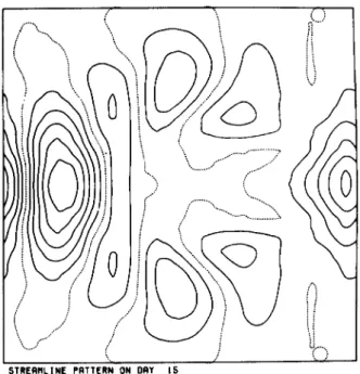
STRERflLlNE PATTERN ON OAY 15

Figure 3(a). Instantaneous disturbance streamlines on day 15, for the sine wave block experiment.

D I V OF EDDY POT. VORT FLUX 15-21ml.Ell

747

Figure 3.1:Instantaneous eddy flowψ1for a dipole block. The dipole block locates at the center of this panel. The contour interval is arbitrary. After Shutts (1983).

20

(23)

Chapter 4 Case study: Trajectory analysis

A trajectory analysis is demonstrated how air parcels move in a Lagrangian manner during the blocking maintenance. Although there have been some previous studies using trajectory analyses (Crum and Stevens 1988; Croci-Maspoli and Davies 2009), they are all done for the blocking formation (onset), i.e., to investigate origins of air of blocking anticyclones. In this study, trajectories originating from synoptic anticyclones and cyclones upstream of blocks are calculated for investigating the interaction between blocking and synoptic eddies.

Ten blocking events are selected in winter (November to April) during 1990 to 2005.

Five events are chosen in each eastern Pacific and Atlantic region, where blocks most frequently occur (e.g., Pelly and Hoskins 2003b; Schwierz et al. 2004; Barriopedro et al.

2006). These Pacific and Atlantic events will be abbreviated as ‘PAC’ and ‘ATL,’ respectively.

The analysis is carried out by using Ertel’s PV (hereafter PV) and the wind with horizontal resolution of about 1.125^◦×1.125^◦(320×160 Gaussian grids) and time resolution of 6 hours. The data used are the Japanese 25-year ReAnalysis (JRA-25) and Japan Me- teorological Agency Climate Data Assimilation System (JCDAS). The vertical level for the analysis is an isentropic surface of 320 K, where the activity of synoptic eddies shows the maximum in the vertical direction (refer ahead to Fig. 8.1b). This level nearly corresponds to the tropopause (also refer ahead to Fig. 8.1d). It is also found that the amplitude of blocking is the maximum in the upper troposphere (Dole 1986).

Then, quantities are decomposed into synoptic eddy and blocking components by

(24)

using a time filter. The Lanczos filter with a cutoﬀperiod of 8 days is used; the high- and low-frequency components correspond to synoptic eddies and blocking flow, respectively.

Blocking and its duration are defined by our own procedure (PV base), which is essentially the same as Pelly and Hoskins (2003b)’s one (potential temperature base). This is based on the fact that blocking is characterized by a consequent reversal of the usual meridional PV gradient (Fig. 4.1a). In this thesis, the blocking is said to occur when the following is satisfied; a blocking indexBdefining this reversal at a longitudeλ0,

B ≡ 2

∆ϕ

∫ _ϕ₀

ϕ0−∆ϕ/2Pdϕ− 2

∆ϕ

∫ _ϕ₀_+∆ϕ/2

ϕ0

Pdϕ ϕ0 =ϕc(λ)+ ∆, ∆ =0^◦,±4^◦,

(4.1) (where P represents PV, ϕ the latitude, ∆ϕ = 30^◦, ϕc(λ) the central blocking latitude) becomes positive over consecutive longitudes∆λ >15^◦in each sector. The Pacific sector is defined for 160^◦E-225^◦E or 200^◦E-265^◦E¹, and the Atlantic sector for 20^◦W-25^◦E. The central blocking latitude at each longitude is defined as the latitude at which the variance of the high-frequency PV averaged in winter (Nov.-Apr.) during 1981-2005 shows the maximum in the Northern Hemisphere.∆is modifications of the central blocking latitude at each longitude. This modification is necessary because of interannual variabilities such as the North Atlantic Oscillation (NAO), the Pacific North American pattern (PNA) and the El Ni˜no-Southern Oscillation (Pelly and Hoskins 2003b). The largest value of B among∆ =0,4, or−4 is adopted at each longitude. The duration is defined as consecutive days for which the above definition is satisfied continuously at each sector. Also, the onset is defined as the first day of the consecutive days.

Total 10 events composed of 5 PAC blocks and 5 ATL blocks are somewhat subjec- tively chosen (Table 4.1). However, all these blocks have large amplitudes and last more than 8 days, according to the above definition.

The calculation method for trajectories is the same as Yamazaki and Itoh (2009).

Parcels put on synoptic eddies upstream of blocking are traced around blocks. Parcel positions are calculated by using the fourth-order Runge-Kutta scheme; the integration

1We found two kinds of the Pacific blocking in this study. One persists over the Aleutian region drifting from its downstream, while the other persists over western America drifting from its upstream. Schwierz et al. (2004) actually showed two peaks of the blocking frequency distribution just upstream and downstream of the eastern Pacific.

(25)

timestep and period are 10 minutes and 5 days, respectively, and the wind (raw wind, i.e., the unfiltered wind) advecting parcels is obtained from the observational data and interpo- lated linearly in time and by cubic-spline in space. It is shown that trajectories of parcels on an isentropic surface in the upper troposphere represents actual tracks of air over about one week (Nakamura, M. 1994; Appenzeller et al. 1996; Peters and Waugh 1996).

The way to put parcels is explained. At an initial time, parcels originating from a synoptic anticyclone (cyclone) are put on grids which have the values of the high-frequency component PV less than−3.0 PVU (more than 3.0 PVU) and of the raw component PV less than 0.50 PVU (more than 8.0 PVU) upstream of blocks. The reason that parcels are put on quite upstream of blocking (Fig. 4.2) is to observetruebehaviors of synoptic eddies around blocking. The detail will be mentioned in Chapter 6. Dates when parcels are put and the parcel numbers are listed in Table 4.2.

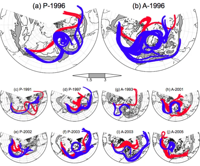
Figure 4.2 shows the trajectories, i.e., behaviors of anticyclonic (cyclonic) parcels originating from synoptic anticyclones (cyclones) around maintaining blocks. Results of P-1996 and A-1996 are explained as representatives. Figure 4.2a for P-1996 shows the trajectories from a synoptic anticyclone (cyclone) existing near the Korean Peninsula at 18 UTC 28 (06 UTC 27) February. Only parcels from the synoptic anticyclone are absorbed into the blocking anticyclone (near the Gulf of Alaska) displayed by a snapshot of the low-frequency PV at 00 UTC 1 March, with rotating anticyclonically. Note that trajectories of the synoptic anticyclone seem to be separated into the north and south directions just west of the blocking anticyclone (near 160^◦W). However, the fact is that only three anticyclonic parcels out of 11 parcels are directed to the south, while the other anticyclonic parcels are absorbed into the blocking anticyclone. It also should be noted that although trajectories of the synoptic cyclone look like passing through the north side of the blocking anticyclone, it is apparent; these parcels keep away from the blocking anticyclone because this anticyclone shifts further south of the displayed blocking when the cyclonic parcels reach there. For A-1996, it is found that trajectories from a synoptic anticyclone and cyclone passing near the Great Lakes at 00 UTC 5 March and 00 UTC 9 March, respectively, are shown in Fig. 4.2b. It can be seen that only anticyclonic parcels

(26)

are attracted toward the Ω-shaped blocking region over the eastern Atlantic (shown by the low-frequency PV field at 00 UTC 9 March), being wrapped up by it. On the other hand, cyclonic ones are repelled by it with drifting downstream. These two events can be said to show the selective absorption of synoptic anticyclones and the asymmetry between synoptic anticyclones and cyclones. The other 8 events also show the selective absorption and the asymmetry in the same manner (Figs. 4.2c-j).

In some events such as A-2005 (Fig. 4.2j), cyclonic parcels are absorbed into blocking cyclones. Furthermore, since even in theΩ-shaped blocks except A-2005, blocking cyclones are temporarily (about half to 2 days) formed at the south side where they are not expressed in the low-frequency PV, it is possible that cyclonic parcels are absorbed by them (e.g., P-2003 and A-2001).

In some events (e.g., P-1996, A-1993, A-1996, and A-2003), there are large differences between the meridional tracks of synoptic anticyclones and cyclones upstream of blocks. The differences would be caused by an effect of theβgyre, i.e., the polar region as a massive cyclone repels/attracts anticyclonic/cyclonic parcels to the south/north by the vortex-vortex interaction, rather than by shifts of the westerly jet, because the tracks of synoptic anticyclones/cyclones systematically shift southward/northward, and jet patterns do not show considerable changes between the two dates when parcels are put on the synoptic anticyclone and cyclone in each event. Such differences also can be seen in results of numerical experiments (Chapters 5 and 6).

Although it can be seen that synoptic anticyclones are absorbed in blocking anticyclones in all the events, the way of the absorption seems different. It may be classified into two manners; i) anticyclonic parcels stay in blocking anticyclones and ii) these parcels pass through the inside of blocking anticyclones, then drifting downstream. Typical former examples can be found in P-1996, A-1996, and P-2003, while typical latter ones in P-1991 and A-2003. The difference between the two manners may be caused by amplitudes of blocking, because the former events have quite low values of the low-frequency PV while the latter does not have so low values. The most typical figures showing this difference are Figs. 4.2a (P-1996) and 4.2i (A-2003). In the former figure the large area

(27)

of low-frequency PV less than 1.5 PVU can be seen, whereas in the latter figure it cannot be seen. Thus, behaviors of synoptic eddies could change due to the strength of blocking.

Effects of diabatic heating are not considered in this study, yet some previous studies suggested that the cloud-diabatic effect contributes to the onset of blocking in some events (Lupo and Smith 1995; Altenhoffet al. 2008; Croci-Maspoli and Davies 2009). However, we think that the adiabatic process is nearly satisfied in our situations, since this study investigates the maintenance process.

(28)

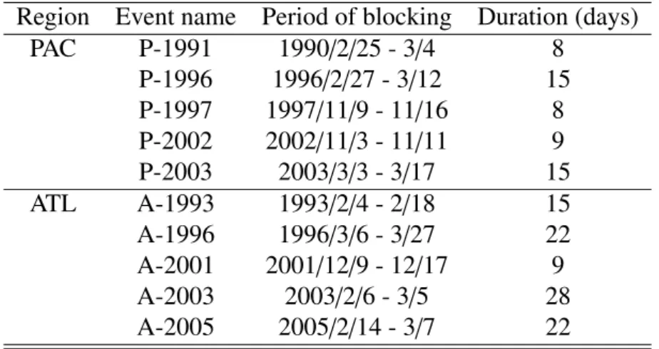
Table 4.1:Regions, periods, and duration of the selected 10 blocking events. Periods are shown in the form of (year/month/day - month/day).

Region Event name Period of blocking Duration (days) PAC P-1991 1990/2/25 - 3/4 8

P-1996 1996/2/27 - 3/12 15 P-1997 1997/11/9 - 11/16 8 P-2002 2002/11/3 - 11/11 9 P-2003 2003/3/3 - 3/17 15 ATL A-1993 1993/2/4 - 2/18 15 A-1996 1996/3/6 - 3/27 22 A-2001 2001/12/9 - 12/17 9 A-2003 2003/2/6 - 3/5 28 A-2005 2005/2/14 - 3/7 22

(29)

Table 4.2:Information of the selected 10 blocking events. (First column) names of the events, (second column) dates [month/day/UTC] when anticyclonic parcels are put and numbers of the parcels, and (third column) the same as the second column but for cyclonic parcels are shown. Note that the number of parcels is diﬀerent between the events because of our unified definitions for anticyclones and cyclones (see text for more details). (Fourth column) dates [month/day/UTC] when low-frequency PV is displayed in Fig. 4.2.

Event name Date (number of parcels) Date (number of parcels) Displayed date for synoptic anticyclone for synoptic cyclone of the blocking flow

P-1991 3/2/00 (5) 2/28/12 (3) 3/3/00

P-1996 2/28/18 (11) 2/27/06 (3) 3/1/00

P-1997 11/12/12 (21) 11/10/00 (23) 11/13/00 P-2002 11/7/00 (16) 11/4/00 (21) 11/7/00

P-2003 3/5/12 (24) 3/9/12 (32) 3/9/00

A-1993 2/13/06 (8) 2/7/06 (3) 2/13/00

A-1996 3/5/00 (20) 3/9/00 (10) 3/9/00

A-2001 12/10/12 (13) 12/9/00 (27) 12/13/00 A-2003 2/16/12 (13) 2/13/18 (14) 2/18/00 A-2005 2/26/06 (17) 2/23/12 (13) 2/26/00

(30)

High PV

Low PV

PV

PV θ=320KPV

(a) ! (b) ! (c) !

High PV!

Low PV!

P_north!

P_south! P on

!=320 K contour!

!"#!$! %! &! '! #! (! )! *! +! $!!

Figure 4.1:(a) PV view of an ATL block. A snapshot of PV on 320 K at 12 UTC 7 February 1993 is shown. The unit of PV is PVU. (b) Schematic representation of the relevant parameters for the blocking indexBat a longitudeλ0. This panel is a modified version of Fig. 2 in Pelly and Hoskins (2003b). See text for details. (c) Distributions of stormtracks and central blocking latitudes ϕc. The + signs show central blocking latitudes, and shades represent the variance of high-frequency PV [PVU²].

(31)

Figure 4.2:Snapshots of blocking flows (PVU, contours and shades) and parcel trajectories from synoptic anticyclones (blue) and cyclones (red) in (a) P-1996 and (b) A-1996. Details about blocking flows and synoptic eddies are described in text and Table 4.2. The other 8 events, (c) P-1991, (d) P-1997, (e) P-2002, (f) P-2003, (g) A-1993, (h) A- 1996, (i) A-2001, and (j) A-2005, are also shown.

(32)

Chapter 5 Numerical experiments

5.1 Channel model

The eddy-feedback eﬀect by the SAM is evaluated by using a β-plane model integrating the equivalent-barotropic quasigeostrophic PV equation, which is the same as S83 and AM02. The basis to use the equivalent-barotropic model is that; i) blocks have vertically coherent structure in the troposphere, and ii) synoptic eddies interacting with blocking are fully mature, becoming barotropic downstream of stormtracks (Simmons and Hoskins 1978; Nakamura and Wallace 1993). To include the asymmetry between synoptic anticyclones and cyclones, the nonlinear equation,

(∂

∂t +U ∂

∂x )

q+J(ψ,q)+β∗∂ψ

∂x = F− E∇²ψ−ν∇⁶ψ, (5.1) is used. Here each symbol is the same as in Chapter 3, butFis the wavemaker forcing,E the Ekman friction coefficient, andνthe hyperdiffusion coefficient. The parameter values except forFandEare the same as AM02;











U =13.8 m s⁻¹,

β=1.6×10⁻¹¹m⁻¹s⁻¹, β∗=1.2βm⁻¹s⁻¹, L_d =845 km,

ν=1.0×10¹⁰m⁴s⁻¹, 2πL_x =42 000 km, πL_y = 21 000 km.

(5.2)

Hereβ∗ = β+U L⁻_D², where the latter term indicates the eﬀect of the Rossby deformation radius of the background zonal flow. The value ofβ_∗here corresponds toL_D =2077 km.

(33)

The numerical integration is performed by the fourth-order Runge-Kutta scheme (time step: 30 minutes). The integration period is 20 days. The initial day is denoted as Day 0, then continuing Day 1, · · · . The meridional and zonal lengths of the channel are 21 000 km and 42 000 km, respectively. Since the boundary conditions are the cyclic boundary in the zonal direction and the rigid walls at the lateral boundary y = 0 and 21 000 km, so that the streamfunctionψis expanded into the following truncated orthonor- mal functions:

F_A_l = cos(ly) ; F_Z^k

l = e^ikxsin(ly), (5.3)

wherek =−K,−K+1, ...,−1,1,2, ...,K,l= 1,2, ...,L, and the truncation wavenumber is K = L=42.

Experimental designs are as follows: A blocking flow is put on the center of the channel at the initial condition, and high-frequency eddies generated by a wavemaker upstream of a blocking drift to the blocking region. As the initial blocking, a modon solution or a rider solution that is a modified form of the modon solution (both solutions together will be sometimes called simply modons) is used. Moreover, we assign three wavemaker settings of diﬀerent meridional positions for each blocking anomaly. After all, six experimental designs are totally used.

The application of modon solutions to blocking cases are first done by McWilliams (1980). The reason why modon solutions are applied to is that they are exact nonlinear solutions of the equivalent-barotropic quasigeostrophic equation and that shapes of modon solutions resemble those of blocks (McWilliams 1980). We do not stress that blocking is just a modon; modons are used in this study because they are the simplest prototype of blocking and their characteristics are well known.

However, there are two problems for this application. First, real conditions are hard to satisfy the existence condition of modons; McWilliams (1980) showed that the climatological monthly mean field does not satisfy this condition. Also, no modons in shear flows is found. Second, modons are unstable forE= 0 (for example, AM02); if blocking is amplified by the instability, we cannot judge which of the unstable amplification or synoptic eddies maintains the blocking. Nevertheless, these two problems can be over-

(34)

come by the following two reasons. First, in a time scale of several days but not a month, the existence condition of modons can possibly satisfied; as this support, Butchart et al.

(1989) investigated the proportional relationship between the PV and streamfunction that is the ground for modons (see Appendix A) for some blocking events, and concluded that this relationship can be satisfied in that time scale over blocking regions. This result implies that the existence condition of modons would be satisfied in that time scale. Second, the unstableness for modons acts for decaying them; Haines and Marshall (1987) showed that a modon loses its energy by Rossby wave radiation into downstream. Also, as will be shown later in our experiments, withE = 0 and unforced conditions, modons are dissi- pated (by Rossby wave radiation) and then drift downstream. The same can be said about rider solutions and spherical modon solutions (described in the next subsection), because both of them have almost the same characteristics as modon solutions (e.g., Appendix A;

Swenson 1987; Neven 2001). From the above, it is plausible to adopt modons as blocking flows in eddy-feedback models.

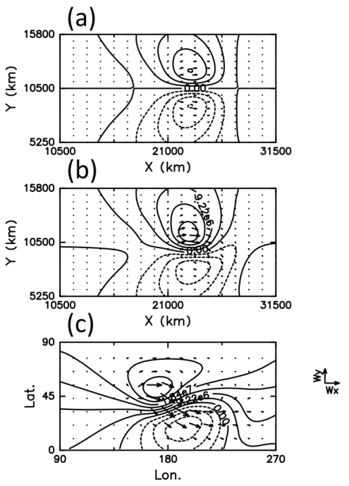
A modon solution and a rider solution are given for the initial values of the dipole-type andΩ-type blocks, respectively (Figs. 5.1 and 5.2). The reader may think that the rider solution is not a pureΩ-type block because of its cyclonic anomaly. Nevertheless, this solution is applied, because i) when we add a constant zonal westerly to the streamfunction field (Fig. 5.2b), then it looks more like aΩ-shape, ii) rider solutions are also the exact solutions of the equivalent-barotropic quasigeostrophic equation (Flierl et al. 1980), and iii) the composite map of the ten events in Chapter 4 looks like a rider solution pattern (see the pattern of composite observed PV in Fig. 7.1)¹. The derivation of modon and rider solutions is described in Appendix A. The same parameters for these solutions as AM02 and Haines and Marshall (1987) are given; ˆc = −U is the intrinsic phase speed, a = 2430 km is the radius of the modon, d_in = 3.9×10⁻¹²m⁻². As one more parameter for the rider solution, a constant PV valueQ= 2.064×10⁻⁵s⁻¹called ‘rider’ is given in the region ofr≤a(ris the radius from the modon center).

1The author think that a rider solution-like structure can appear during blocking duration since shapes of the blocking change between the dipole-shaped and anticyclonic monopole-shaped during the duration.

Therefore, we could defineΩ-type blocks as rider solutions which are the hybrid structure of the anticyclonic monopole and the dipole structure.

(35)

The wavemaker is basically put in the region centered at 7875 km upstream of the block as

F = 

F˜sin{_π_(x₋_x

0)

∆x

}cos{₄_π_(x₋_x

0)

∆x −ωt}

sin{_π_(y₋_y

0)

∆y

} forx₀< x< x₁andy₀ < y<y₁,

0 otherwise, (5.4)

where ∆x = x₁ − x₀ = 10 500 km; ∆y = y₁ − y₀ = 2625 km; ˜F = 5.40× 10⁻¹⁰s⁻²; (x₀,y₀)= (5250,9187.5) km, which correspond to an eddy diameter of 2625 km with an amplitude as large as or less than the amplitude of the initial blocking, and the period ω/2π = 4.5 days. Our experiments examine how eddies generated by the wavemaker interact with the blocking. In these experiments, the blocking duration is checked in the following three wavemaker settings; i) no wavemaker is put (No-eddy Exp), ii) the above wavemaker is put (No-shift Exp), and iii) the wavemaker is shifted 1000 km southward from that of the No-shift Exp (Shift Exp). Note that this shift is much larger than that in AM02 (about 400 km).

To determine the value of the Ekman friction coeﬃcientE, a linear stability analysis is made. This analysis checks whether a blocking flow is stable or not. Details of equations and procedures are described in Appendix B. Results are shown in Fig. 5.3. Both the blocking flows, modon and rider solutions, are unstable for E < 0.24 day⁻¹. Then, the reader may think that experiments should be taken under stable conditions of E ≥ 0.24 day⁻¹. However, in these conditions the blocking duration and the eddy-feedback eﬀect are not evident due to too strong damping. Hence, the value ofE = 0.09 day⁻¹ is chosen for our experiments; for this value the interaction between blocking and eddies is not contaminated by damping, and this instability for the blocking flows does not act for their maintenance but their decay. Note that similar results are obtained for any (larger or smaller) values ofE, as mentioned later.

The reason why the unstableness of the modon and rider solutions acts for their decay may be as follows: Patterns of unstable modes similar to the blocking ones are only the 14th and 15th modes for the modon solution (not shown). Since these modes have the 2 smallest growth rates (Fig. 5.4a), they probably do not dominantly contribute to the blocking flow. On the other hand, both the patterns of the fastest growing modes for the modon and rider solutions are largely diﬀerent from the initial blocking patterns, thereby

(36)

decaying them (Figs. 5.4b and c).

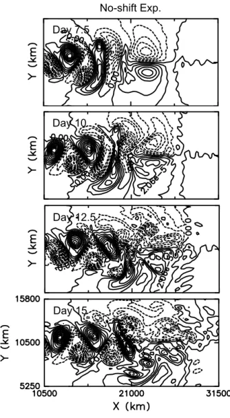
Time evolutions of the dipole blocking in No-eddy, No-shift, and Shift Exps are shown in Fig. 5.5. In No-eddy Exp (Fig. 5.5a), the block cannot maintain its amplitude and then is drifted downstream by the background flow (note that the blocking center on Day 0 is x = 21 000 km.), because its energy is carried out downstream by the Rossby wave radiation, which is manifested by the wave activity flux (Fig. 5.6a). On the other hand, in the time sequence in No-shift Exp, we can see the absorption of eddies into the blocking, that is, anticyclonic/cyclonic eddies are attracted and absorbed by the blocking anticyclone/cyclone. This absorption is easily recognized, for instance, during Day 10 to Day 12.5, since the anticyclonic eddy (tagged with the star mark) just upstream of the block on Day 10 moves northeastward in a short time scale of 1-2 days. Behavior of the absorption can be more obviously seen in the PV field (Fig. 5.7), because there is the scale eﬀect between PV and streamfunction (Hoskins et al. 1985), which means that the PV field shows a clearer view than the streamfunction field obtained by the inverse Laplacian to PV. Since the same feature is also seen on other days and in Shift Exp, the selective absorption of eddies by the blocking vortices with the same polarity can be confirmed. In both No-shift and Shift Exps, the block keeps large amplitudes and is not strikingly drifted downstream even on Day 15. Furthermore, even compared with No-shift Exp, the meridional position of the block in Shift Exp is remarkably locked on that day. The above results are consistent with the SAM predicting that the eddy-feedback can be accomplished independent of meridional shifts of a wavemaker (Chapter 3).

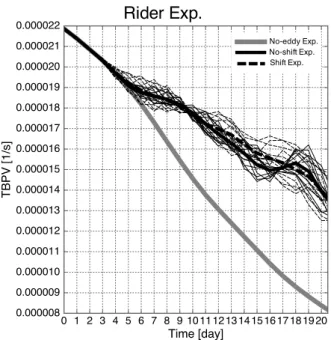
To objectively quantify the blocking duration, we define the total blocking PV (hereafter referred to as TBPV) as a retention rate of the blocking PV at the initial blocking position. The definition of the TBPVq_blockis

q_block= 1 S

∫

S

(q_S −q_N)dS, (5.5)

where S is the initial blocking interior area, q_S positive values of q in the region of the initial streamfunction ψinit < −9.225× 10⁶m²s⁻¹, and q_N negative values of q in ψinit > +9.225×10⁶m²s⁻¹. The sum of these two regions corresponds toS, that is, the inner regions of the outermost solid and dashed contours represented as the thick lines in

(37)

Fig. 5.1. In addition, to consider the phase dependence of synoptic eddies, integrations with diﬀerent initial phases of the wavemaker are carried out, and the average of these ensemble members is taken (Arai 2002). Thus, phase-independent time evolutions are obtained. Here, the forcing term in (5.4) is replaced by

F = F˜sin

{π(x−x₀)

∆x }

cos

{4π(x−x₀)

∆x −ωt−ϕ }

sin

{π(y−y₀)

∆y }

, (5.6)

whereϕis a phase factor. By changing the phase factorϕbyπ/5 in the range of 0≤ ϕ <

2π, 10 integrations are performed. Time changes of the TBPV for the ensemble members and averages in No-shift and Shift Exps are illustrated in Fig. 5.8.

This figure shows that the eddy-feedback can occur even when there is a large shift of the wavemaker. We can see in both No-shift and Shift Exps that the TBPV of the ensemble means keeps almost the same values from Day 5 when the first eddies arrive at the block to about Day 10. The TBPV of some members in Shift Exp has almost the same value as the ensemble mean in No-shift Exp. As to the phase-dependency, since all the ensemble members in each Exp have much larger TBPV than that in No-eddy Exp, the eddy-feedback does not depend on the longitudinal phase of the wavemaker. These results objectively support the blocking maintenance by the SAM. Here, behaviors of upstream eddies should be pointed out; anticyclones/cyclones shift southward/northward from the mean stormtrack due of theβ gyre effect (Figs. 5.5b and c). This shift has a tendency to reduce the TBPV value. Nevertheless, the effect of the selective absorption overcomes this shift effect, maintaining the large TBPV value.

From here, evolutions of the Ω-type block are analyzed (Fig. 5.9). Also in this case the selective absorption is evident. The stationarity and amplitude of theΩ-type block are stronger than those of the dipole-type block. This can be explained by the characteristic that the larger amplitudes of blocking are, the stronger the vortex-vortex interaction becomes (Chapter 2). Since the blocking anticyclone of the rider solution is stronger than that of the modon, the SAM more eﬀectively works for the Ω-type than the dipole-type block. Figure 5.10 shows the time changes of the TBPV for theΩ-type block. Although the decay is somewhat faster than that of the dipole-type block (note that the initial amplitude of the TBPV is diﬀerent from that of the dipole type), this reflects the faster decay in

(38)

No-eddy Exp (see also Figs. 5.6 a and b). Therefore, the diﬀerence in the TBPV between No-eddy Exp and No-shift (or Shift) Exp is almost the same as that for the dipole-type block, and the blocking is well maintained by the eddy-feedback against dissipation and wave radiation. Also, the spread in both Exps is still small. In addition, we can point out that the two TBPV values of the ensemble means in the No-shift and Shift Exps are quite the same. This feature probably indicates that the stronger blocking anticyclone than that of the dipole-type tends to fix its position (the phase lock of blocking, see Chapter 2).

There is a diﬀerence between downstream patterns of the dipole-type and Ω-type blocks; comparing the panels of Day 12.5 or Day 15 of No-shift and Shift Exps in Fig. 5.5 with those in Fig. 5.9; for the dipole-type block downstream small anticyclones (pointed by the left-directed arrows) permeate from the blocking anticyclone, whereas for theΩ- type the blocking anticyclone traps the downstream anticyclones so as to keep a large scale until those days. Such permeability may reflect the diﬀerence between the behaviors of anticyclonic parcels passing through and wrapped up with blocking anticyclones, discussed in Chapter 4.

We take, to make sure, the same experiments for E = 0.25 day⁻¹ in which the linear stability is satisfied (see Fig. 5.3). Then, similar results are obtained but with very fast damping of the blocks (not shown). Although the way of the blocking decay is diﬀerent by the Ekman friction or by the unstableness of the modon or rider solution, the SAM works for the block maintenance against any values ofE.

Finally, the PV supply rate predicted by the SAM will be verified. In the SAM, the strength and amount of supplied PV are important; it is expected that, since the size and strength of the wavemaker aﬀect the amount and strength of PV supplied to the block, respectively, their increases improve the maintenance of the blocking. Then, we perform sensitivity analyses for amplitudes and sizes of the wavemaker to the dipole-type blocking in No-shift Exp. To begin with, experiments with diﬀerent sizes of the wavemaker are performed; in addition to the standard experiment with the eddy diameter of 2625 km (R2625), the diameter size is replaced as 2100 km (R2100) or 1750 km (R1750). Figure 5.11a shows that the TBPV increases as the size of eddies does. The next experiment is

(39)

to change amplitudes of the wavemaker; the standard value of ˜F = 5.40×10⁻¹⁰s⁻² (F1) are replaced as 1/2 (F1/2), 1/4 (F1/4) or 1/8 (F1/8) times the amplitude of ˜F. Figure 5.11b shows that the stronger the amplitudes are, the larger the TBPV are. These results are consistent with the PV supply mechanism of the SAM. Concerning the spread, the experiment with the largest eddy amplitude or size has the largest spread because eddies also move the blocking vortex (not shown), but it is still small compared with the value of the TBPV. Hence, we can say again that the phase-dependence does not contaminate the eddy-feedback.

Since it is shown in the above experiments that the eddy-feedback mechanism in the SAM is robust, the hypothesis that blocking flows themselves determine their longevity suggested by S83 and Pierrehumbert and Malguzzi (1984) is consistent with the SAM.

Moreover, in the SAM, the configuration of blocking flows can be chosen flexibly, because the condition requested to the maintenance is only that blocking is a stationary anticyclone with a large amplitude, which can interact with synoptic eddies. In fact, even when similar experiments are performed using modon and rider solutions with diﬀerent parameters and a Gaussian vortex, i.e., an anticyclonic PV anomaly given by the Gaussian distribution, consistent results are obtained. Experiments with the channel twice as wide as that of the above are also performed and the same results can be obtained.

5.2 Spherical model

Modon solutions on a β-plane are extended to those on a sphere, that is, spherical modons. On a sphere, dipole vortices of the modon become asymmetric because of the constraint of angular velocity (Neven 1994). We will show results from numerical experiments with the same design as in the channel model but for spherical modons as the initial block through this subsection.

A spherical modon solution as the initial block is adopted from Verkley (1984) and Neven (2001). This solution, its derivation, and its parameters are found in Appendix A.

As for the parameters, the outer wavenumber of the modonn_out = 1, the inner wavenumber of the modonnin = 10, and the modon radiusθa = 21.15^◦are adopted because these

(40)

parameters give a similar amplitude and size to those of theβ-plane modon solution. The center latitude of the modon is put on 45^◦N. With these parameters the spherical modon solution is shown in Fig. 5.12. Note that this figure is displayed in streamfunction, and then the north-side anticyclone will be further highlighted in geopotential height. The north-side anticyclone can also be highlighted by using a polar-stereo projection (Fig.

5.12b) or with a background westerlyU_ssuperimposed (Fig. 5.12c).

For spherical-model experiments a spectral model with the triangular truncation at wavenumber 42 (T42) is used. The governing equation on the sphere becomes

(∂

∂t + U_s R

∂

∂λ )

q+J(ψ,q)+βs

1 R

∂ψ

∂λ = F− E∇²ψ−νH

(

∇⁸− 2⁴ R⁸ )

∇²ψ (5.7) (U_s, the background zonal wind speed at the equator;λandϕare longitude and latitude, respectively; R = 6371 km, the radius of the sphere; βs ≡ (2/R² +1/L²_D)U_s+2Ω; Ω = 7.29 × 10⁻⁵s⁻¹, the angular velocity of the sphere; νH, the hyperdiﬀusion coeﬃcient), which is the same equivalent-barotropic quasigeostrophic PV equation as the channel- model equation. The parameter values of L_d = 822 km and νH = 2.1×10³⁵m⁸s⁻¹ are set, and the other parameters are given the same values as the channel model except for U_s = 19.52 m s⁻¹ with which the background zonal flow is 13.8 m s⁻¹ at the mid latitude (45^◦N), coinciding withU in the channel model.

The wavemaker is put in the same way and has the same amplitude and size as the channel model, but only the meridional shift is diﬀerent; the southward 10^◦ shift (Shift Exp) and, in addition, the northward 10^◦shift (N-shift Exp) due to the north-south asymmetry of the spherical model. Then, time evolutions in these Exps are examined.

The time evolution of No-eddy Exp shows that before Day 10 the blocking anticyclone already loses its vortex-like structure, and then on Day 15 this becomes rather zonally uniform (Fig. 5.13a). This is caused by strong Rossby wave radiation from the blocking because of the spherical geometry. This can be confirmed by the wave activity flux (Fig.

5.6c) which is a indicator of strong Rossby wave radiation (e.g., Takaya and Nakamura 2001). Stronger wave activity flux can be found for the spherical modon than those for the channel modons (Figs. 5.6a-c). In No-shift Exp, on the other hand, we can see that the initial blocking pattern still remains even until Day 15 (Fig. 5.13b). Thus, the diﬀerence

(41)

between the blocking duration of No-eddy and No-shift Exps is more distinct than that on theβ-plane. The time evolutions of Shift and N-shift Exps (Figs. 5.13c and d) show that the maintenance of the initial blocking position and amplitude can be seen on Day 10 and Day 15. Of course, in every experiment with the wavemaker forcing, the absorption of anticyclonic eddies into the blocking anticyclone occurs (not shown). To conclude from the above results, the SAM on the sphere works more profoundly than on theβ-plane and to make the blocking structure realistic.

In the spherical model, we have chosen the parameter values of the modon solution or the value of the Rossby deformation radius in an arbitrary manner, to some extent. Then, we perform the same experiments with diﬀerent values that are not largely diﬀerent from the above parameters. Results from these experiments are essentially the same. The phase dependence of the wavemaker is also checked, yet similar results are obtained.

(42)

(a) Dipole-type (b) Ω-type 図3:

Figure 5.1:Initial streamfunction of (a) the dipole-type and (b)Ω-type blocks. The contour interval is 9.225×10⁶m²s⁻¹and dashed lines show negative values. The zero contour is omitted. The interior of the outermost thick lines is the areaS to calculate the total blocking PV (TBPV) defined in (5.5).

40

(43)

(a) Dipole-type (b) Ω-type 図3:

(a) Dipole-type (b) Ω-type

図4:

Figure 5.2:Same as Fig. 5.1 but for the streamfunction fields with the background zonal windU.

The zero contour is displayed.

41

(44)

Figure 5.3:Fastest growth rate [day⁻¹] of the modon (circle) and rider (triangle) solutions as a function of the Ekman friction coeﬃcientE[day⁻¹].