Using a Renormalization Group to Create Ideal Hierarchical Network Architecture with Time Scale Dependency

(1)

INVITED PAPER

Special Section on Frontiers of Information Network Science

Using a Renormalization Group to Create Ideal Hierarchical Network Architecture with Time Scale Dependency

Masaki AIDA^†a),Member

SUMMARY This paper employs the nature-inspired approach to investigate the ideal architecture of communication networks as large-scale and complex systems. Conventional architectures are hierarchical with respect to the functions of network operations due entirely to implementation concerns and not to any fundamental conceptual benefit. In contrast, the large-scale systems found in nature are hierarchical and demonstrate orderly behavior due to their space/time scale dependencies. In this paper, by examining the fundamental requirements inherent in controlling network operations, we clarify the hierarchical structure of network operations with respect to time scale. We also describe an attempt to build a new network architecture based on the structure. In addition, as an example of the hierarchical structure, we apply the quasi-static approach to describe user-system interaction, and we describe a hierarchy model developed on the renormalization group approach.

key words: large-scale and complex systems, renormalization, adiabatic approximation, local interaction, hierarchical structure

1. Introduction

Information and communication networks are the world’s largest systems in the terms of both the number of devices connected and their spatial extent. Also, by considering en- vironmental changes such as the deepening of ties with society and the diversification of applications, we can regard the networks as large-scale and complex systems. How can we design and operate such large-scale and complex systems appropriately? What design principles are required? Before starting concrete discussions, it is necessary to explain the standpoint of this paper [1].

1.1 Networks as Large-Scale and Complex Systems The most well-known large-scale and complex system is our world. The number of components that form this world and their diversity readily confirm that it is the ultimate large- scale and complex system. So why is this ultimate large- scale and complex system, the world, stable? We believe that the world will still exist tomorrow and that the sun will rise tomorrow just like the past. Even though we know that no prior state is ever repeated exactly at the scale of atoms or elementary particles that make up our world, we believe that the world is stable. Such orderly behavior of the world is created through so-called self-organization, synergy effect, or collective phenomena of fundamental structure. This

Manuscript received September 6, 2011.

Manuscript revised December 22, 2011.

†The author is with the Graduate School of System Design, Tokyo Metropolitan University, Hino-shi, 191-0065 Japan.

a) E-mail: maida@sd.tmu.ac.jp DOI: 10.1587/transcom.E95.B.1488

framework is interesting and gives useful intention to engineering. The question of where the stability or orderly behavior of the world comes from, probably corresponds to the following questions. Assuming that God created the world, whatholy secrets(orgimmicks) were used at the Creation to yield the orderly behavior of the world? Conversely, even if we assume that God does not exist, what are thegimmicks that make us feel that somethingis behind the orderly behaviors of the world?

This paper discusses one part of a research project that is examining suchgimmicksand focuses on the design of information communication networks as large-scale and complex systems. In other words, the aim of this research is as follows. Engineering systems are created by humans, who consciously or unconsciously imitate the Creation of the world by God. Our goal is to create a design approach that can produce large-scale complex systems that autonomously create well-ordered behavior. In this context, we discuss the need for a network architecture based on a hierarchical structure; its network operations exhibit time scale dependencies. In addition, we focus on the relationship between the user and the system as a typical example of the hierarchy, and discuss how to design the hierarchy by using a renormalization group.

1.2 Where Does the Well-Ordered Behavior of the World Come from?

The question of what are the gimmicks that stabilize the world can be answered in various ways. For example, one explanation based on the anthropic principle is as follows.

First of all, the stability of the world allows the emergence of intelligent life like human beings, and our existence allows the world’s stability to be discussed. So, the question about why the world is stable can arise only in a stable world, sug- gesting that the question is some form of tautology.

Of course, we cannot give a complete answer about the gimmickssince the natural mechanisms are not completely understood. However, since our purpose is not to understand nature but apply some form ofgimmicksto engineering systems, we can try the currently consideredgimmicks to evaluate their usefulness for engineering. In this paper, we consider the following twogimmicks.

• Action through a medium (Local interaction) [2]

In physical systems, there are two concepts that describe the interactions that can occur between two objects oc- Copyright c2012 The Institute of Electronics, Information and Communication Engineers

(2)

cupying diﬀerent positions; action at a distance and action through a medium (local interaction). The former yields a model in which two widely-separated objects interact directly. The latter does not permit the existence of direct interaction between widely-separated objects; it assumes that interaction occurs only between spatially- adjacent objects, and the eﬀect of interaction is gradually exchanged between the objects. Modern physics supports the action through medium concept, so interaction occurs locally. In such a model, space is filled with physical quantities at all points (which forms a field), and any variation in the physical quantity at a point would propagate through the field at finite speed.

• Renormalizability (Reducing the degrees of freedom in dynamics)

When attempting to observe a massive aggregation of extremely small objects that interact in complex ways, we can more easily comprehend the aggregate (or system) by reducing either the temporal or spatial resolution (or both), i.e., coarse graining transformation. In renormalization theory, complex systems are understood by observing changes in a measurable attribute identified by the coarse graining transformation. The coarse graining transformation of observations is called the renormalization transformation. We consider a system that exhibits large (or infinite) degrees of freedom at the microscopic scale. If the system is well described by small (or finite) degrees of freedom at the macroscopic (measurable) scale through renormalization transformation, the system is called renormalizable. While the renormalization theory has many brilliant successes in various fields of physics, it must be customized for each problem. That is, there is no general analytical method that can be freely applied in various fields [3].

In the action through a medium concept, an object in- teracts only with its neighbors, at any instant. In the world of action at a distance, the action of an object instantly influences all places, including the end of the universe, and conversely the action of any object, regardless of its location, instantly influences the object. In this situation, the components of world are associated with each other very strongly, which might limit the flexibility of the world. Therefore, the action through a medium concept appears to be a keygim- mickin producing stable systems, while ensuring the freedom of local action.

Even if we do not fully comprehend the attributes of micro-components such as atoms or we do not understand the complete mechanisms of nature, we can admire the orderly behavior of the world. This means that even if there are huge degrees of freedom when the world is observed at the micro-scale, almost all degrees of freedom are missing at the human perceptible macro-scale, and only a small number of macro parameters are needed to describe the world.

This confirms therenormalizabilityof the world.

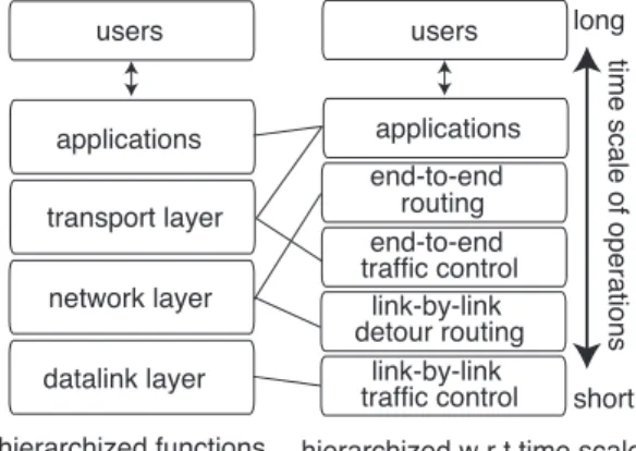
Fig. 1 An example of hierarchical architecture exhibiting time scale depndency.

1.3 Related Work

The conventional architecture has a hierarchical structure with respect to functions of network operations, but it might not have any fundamental justification, only implementation benefits. In contrast, the large-scale systems found in nature exhibit hierarchies that are space/time scale dependent;

these hierarchies underlie the orderly behavior of the systems. In this paper, we assume that the hierarchy concept is the key to designing and operating large-scale and complex systems. In order to apply this concept to engineering systems, we adopt the nature-inspired approach [1], [4].

Figure 1 shows an example of the hierarchical structure of network control mechanisms that yield operations with time scale dependency. For example, TCP, a protocol of the trans- port layer, includes functions acting on wide range of time scale. Window flow control acts around round trip time, and exponential backoﬀ sometimes acts around dozens of sec- onds. These functions might be split into diﬀerent layers of time scale.

As another approach for designing network control methods inspired by phenomena in nature, the bio-inspired approach has been actively studied [5]–[7]. Reflecting the diversity of biological phenomena, the bio-inspired approach covers a wide variety of applications of network issues, but the relevant technology is self-organization to form autonomous structures. The typical example of self- organization in the bio-inspired approach is the reaction diffusion model, which is based on the Turing pattern. This model demands that the values of several parameters be tuned, but this is diﬃcult to do in general networks. In addition, the interaction between two diﬀerent state variables is required, but this yields long convergence times.

Renormalization groups for communication networks have been studied for evaluating the scalability of routing protocols; this requires the introduction of a renormalization transformation of the network topology [8]. However, networks with hierarchical structure have not been discussed.

The rest of this paper is organized as follows. Sec- tion 2 starts with an overview of the network architecture

(3)

based on our nature-inspired approach. After discussing the hierarchical structure with spatial and temporal dependencies, we show a design approach for the hierarchy layers.

Also, we explain the quasi-static approach, which describes the interaction between user and system, as an example of the inter-hierarchy layer design process. Section 3 shows the design of a hierarchical structure based on the renormalization group. After introducing the notion of renormalization, we explain the quasi-static approach on the basis of the renormalization group. Section 4 clarifies the structure of the quasi-static approach by using adiabatic approximation and perturbation of non-adiabatic eﬀects. We conclude this paper in Sect. 5.

2. Network Architecture Based on Natural Order In this section, based on two gimmicks introduced in Sect. 1.2, we briefly outline a network architecture with hierarchical structure with time scale dependency. Next, we introduce concrete examples of action through a medium (local-action theory) and renormalization.

2.1 Hierarchical Structure with Time Scale Dependent Network Operations

Various systems in nature exhibit well-ordered behavior due to their hierarchical structure with spatial and temporal scale dependencies. In this paper, we assume that the twogim- micksintroduced in Sect. 1.2 are essential for producing the stability and well-ordered behavior of large-scale and complex systems. Here, we briefly describe the outline of the relationship between the twogimmicksand the hierarchical structures of network systems.

For simplicity of discussion, let us consider a one- dimensional space. Let p(x,t) be a (density) function of position x and time t. This function represents the state or performance at each position, andxdenotes the logical or physical position in the network^†. We assume that the change in the value of the density function at each point is caused only by the migration of the quantity considered, the quantity is never created nor annihilated in the network^††. The temporal evaluation equation, the master equation, is written as

∂

∂t p(x,t)=− _∞

−∞

w(x,r,t)p(x,t) dr +

_∞

−∞

w(x−r,r,t)p(x−r,t) dr, (1) wherew(x,r,t) is the transition rate per unit of time, and its transition is fromxtox+rat timet. Here, we introduce the n-th order moment ofw(x,r,t) with respect to transitionras

cn(x,t) :=

_∞

−∞rⁿw(x,r,t) dr, (2) and use Taylor expansion f(x−r) =e⁻^r^∂x^∂ f(x) of function f(x). The temporal evolution of p(x,t) is given by infinite

series of spatial derivatives as

∂

∂t p(x,t)=^∞

n=1

(−1)ⁿ n!

∂ⁿ

∂xⁿcn(x,t)p(x,t). (3) This is called Kramers-Moyal expansion [9]．Since the series on the right side of (3) contains spatial derivatives of infinite order, the evolution ofp(x,t) at pointxis influenced by the state ofp(x+r,t) at other pointsx+r, simultaneously.

Note that since this is true for any value ofr, (3) includes effects such as action at a distance. In order to eliminate the eﬀect of action at a distance, let us consider the truncation of the series at some finite order. If the series is truncated (that is, we can find somen0such thatcn(x,t)=0 for alln>n0), then the series only includes spatial derivatives of finite order, and thus the temporal evolution ofp(x,t) is determined only by information in the infinitesimally close neighborhood ofx^†††. This corresponds to action through a medium.

Therefore, according to the concept of the action through medium, we would be dealing with models based on partial diﬀerential equations or diﬀerence equations, inevitably.

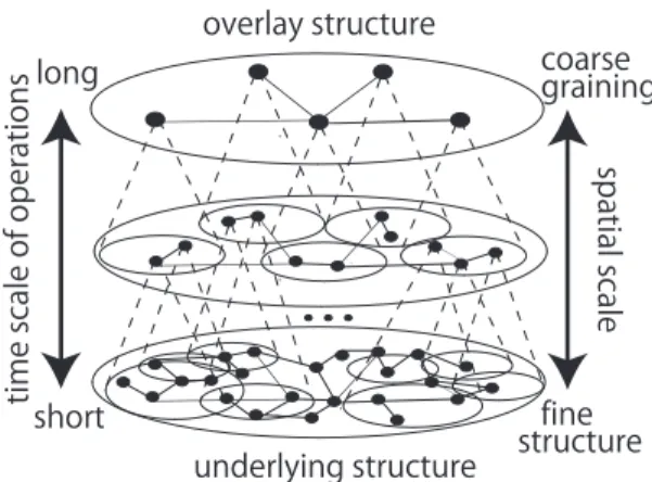
In network systems, action through a medium or local interaction is a notion used for convenience, and of course the range of local interaction is not infinitesimal in the mathematical sense. Local interaction at a certain time scale requires the following three factors: local information that can be collected without degradation in information fresh- ness, neighborhood (the corresponding spatial range), and autonomous interaction with the neighborhood based only on the local information. Therefore, local interaction can be defined in each time scale and it might not seem local if we observe it at microscopic scale (Fig. 2)．

One of most elegant and mysterious facts in nature is that systems having diﬀerent microscopic structures occa- sionally exhibit the same macroscopic behaviors. This is referred to as the universality of natural phenomena [3]．

As an example of the universality, the diffusion equation in Sect. 2.2 can cover various diffusion phenomena (for example, heat flow in solids, the density of ink in the liquid, and the density of gas in the air). The only difference is found in the value of a constant (the diffusion coefficient) and difference in the microscopic structure is reflected in the value of the diffusion coefficient. In this sense, we can recognize that this type of temporal evolution equation shows the time scale decomposition of hierarchical systems. Indeed, this decomposition itself enables us to recognize that the world is stable. The form of the temporal evolution equation describes the phenomena present at the observed time scale

†As shown in Sect. 2.3, xdenotes the position in abstract parameter space.

††Generalization to include creation and annihilation is easy.

However, if we introduce them now, we cannot distinguish creation/annihilation from teleport, that is a typical non-local eﬀect.

†††Since the structure of networks is discrete, the diﬀerential equation becomes a diﬀerence equation. In this situation, the term of higher-order derivative requires information of far distant components even if it is finite-order. A discrete model based only on local information is discussed in Sect. 2.2.

(4)

Fig. 2 Hierarchical structure of networks with temporal and spatial scale dependencies: The range of local interaction is not local if we observe it at a more microscopic scale.

and effects from more finely granular structures are reduced and represented as the value of the coefficient. In contrast, the effects from longer time scales impacts the initial and the boundary conditions of the equation.

From the above discussion, in order to compose the hierarchical network architecture with time scale dependencies, we need to resolve the following two issues:

• Designing action rules for each layer of the hierarchy Let us consider, for a certain time scale, a control action based only on local information where actions influence only the neighborhood. In order to establish the concrete control action, we need to develop a framework of autonomous distributed control based on action through a medium. That is, the action rule in a certain layer should be described by a partial diﬀerential equation.

• Understanding the mutual interaction of layers in the hierarchy

Let us consider a situation observing phenomena of shorter time scale. In order to understand the mutual influence between actions at different time scales, we need to know the appearance of the phenomena at longer time scales. That is, the coefficients of the partial differential equation, that describes the action rule, should be determined so as to reflect effects of the underlying layer. This procedure requires us to develop a renormalization theory customized for networks.

In the following two subsections, we show examples of these issues, respectively.

2.2 Local Interaction and Autonomous Distributed Con- trol

Here, we explain the design of an autonomous distributed mechanism for network control, based on local interaction using the diﬀusion phenomena as an example. Assuming the change in density functionp(x,t) occurs only with continuous flow, i.e., we can ignore creation, annihilation, and jump to other position, thenp(x,t) satisfies the continuous equation,

∂p(x,t)

∂t =−∂J(x,t)

∂x , (4)

whereJ(x,t) denotes a one dimensional vector representing the flow amount of p(x,t) that moves throughxper unit of time. In diﬀusion, the flow is from higher density side to lower density side, and flow strength is proportional to the gradient of the density, so we have

J(x,t)=−κ∂p(x,t)

∂x , (5)

whereκis a positive constant and is called the diﬀusion co- eﬃcient. By substituting (5) into (4), we have the temporal evolution equation ofp(x,t) as follows:

∂p(x,t)

∂t =κ∂²p(x,t)

∂x² . (6)

This is the well-known diffusion equation. Diffusion is a common phenomenon seen everywhere in nature. Surpris- ingly, an extremely wide variety of diffusion phenomena can be described by the diffusion Eq. (6), as explained in the pre- vious subsection. The complex microscopic structure characteristic of each phenomena is reduced, and the characteristics of each phenomenon are expressed by the small number of parameters (in this case, only one parameter).

For the initial condition p(x,0) = p₀(x), (6) has the following solution.

p(x,t)= _+∞

−∞ N(x−y,2κt)p0(y) dy, (7) whereN(x, σ²) is the density function of the normal distribution with mean 0 and varianceσ², that is,

N(x, σ²)= 1

√2πσ²e⁻^x

2

2σ2. (8)

The physical meanings of (7) are simple. The density function at the initial state at each point diﬀuses, over time, in accordance with the normal distribution, and the solution is the superposition of the density functions.

As seen in this example, from an engineering standpoint, the behavior of systems based on action through a medium (local interaction) can be associated with the framework of autonomous distributed control [1], [2]. The state of the entire system exhibits orderly behavior as described by the solution (7) of the differential Eq. (6), even though all subsystems autonomously act based only on their local information, as (5), and nobody knows the information for the entire system. Applications of autonomous control using the diffusion phenomenon include traffic control for congestion avoidance and load balancing systems [2], [4], [10], [11].

The recipe of the framework of autonomous distributed control based on local interaction is summarized in Fig. 3. If the behavior of subsystems is properly designed at a microscopic scale, this framework allows us to indirectly control the behavior of the whole system at a macroscopic scale [2].

For the example of diﬀusion, we considered a control mechanism that harmonizes the network state by the

(5)

• Let us think about the behavior of state that the whole system has to have ((7) and (9) correspond). Moreover, let us find the partial diﬀerential equation that has the solution that provides such a behavior ((6) and (10) correspond).

• Let us identify the local interaction that the partial diﬀerential equation describes ((5) and (11) correspond). Finally, we design the behavior of subsystems to replicate local interaction.

• As a result, even though the autonomous action of each subsys- tem is based only on its local information, the state of the whole system exhibits the desired behavior as a solution of the diﬀeren- tial equation.

Fig. 3 Recipe for designing mechanisms of autonomous distributed control based on local interactions.

Fig. 4 Renormalization transformation of diﬀusion phenomenon.

smoothing eﬀects of diﬀusion. We can introduce another mechanism that produces spatial patterns of a finite size.

The following procedure is an application of the recipe shown in Fig. 3. First, we define a new functionq(x,t) by using (7) as

q(x,t) :=

√2κe^2ct

σ p

⎛⎜⎜⎜⎜⎜

⎝

√2κe^2ct σ x,e^2ct

⎞⎟⎟⎟⎟⎟

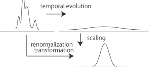
⎠, (9) wherecandσare positive constants. This function is obtained by the procedure that makes the temporal evolution of the solution (7) of the diﬀusion equation exponential against time and simultaneously scales the spatial axis in accordance with diﬀusion, as shown in Fig. 4. The limit distribution is limt→∞q(x,t)=N(x, σ²). This transformation (9) is a sort of renormalization transformation and is discussed in the next section. In accordance with the approach shown in Fig. 3, we can obtain the temporal evolution equation of q(x,t) and the corresponding local-action rule, as

∂

∂tq(x,t)=c ∂

∂xx+σ² ∂²

∂x²

q(x,t), (10) J(x,t)=−c

x+σ² ∂

∂x

q(x,t). (11)

This control mechanism produces a spatial structure whose size depends on the value of parameterσ, and we can apply it, for example, to autonomous distributed clustering mechanisms in ad hoc networks. This mechanism has a desir- able property for application to actual networks. Since the temporal evolution Eq. (10) contains up to the second-order derivative, local interaction requires only local information,

even when the networks are given a discrete structure. In order to enable to apply this control mechanism to any network topology, we have to enhance it so that the local interaction does not depend on the coordinate system [12], [13].

Alternatively, if we restrict the network topology to a regular grid, we can apply Fourier transformation and define a higher-order derivative. By using them, other types of structure formation mechanisms for the restricted networks are possible [14].

2.3 Quasi-Static Approach as an Example of Creating Hi- erarchical Architecture

Let us consider the effect that arises between different layers of the hierarchy. The characteristic whereby the degrees of freedom of a system are reduced when the system is ex- amined at a macroscopic scale is not special in itself, and we can find many examples in natural and engineering systems. Statistical multiplexing effect (economy of scale) in the design of communication channels is one example. If we aggregate a lot traffic flows, the statistical effect tends to decrease the relative variation around the average, and therefore the designs that use the average tend to work well.

In addition to the statistical effects, we would like to take certain networking effects into consideration. The meaning of the networking effectsis as follows. When we try to understand the characteristics of the entire system, one approach is to investigate the details of each component of the system. This concept is called reductionism. The net- working effectmeans the phenomena that cannot be understood through reductionism. That is, the characteristics of each component are not the sole determinant of the characteristics of the entire system, instead we must consider thenetworking effectsgenerated by component interaction.

In this situation, the eﬀects created by the characteristics of each component become weak but the networking eﬀect becomes dominant, and new non-trivial characteristics emerge at the macro-scale.

One example of the above situation is the quasi-static approach; it describes the retry traﬃc generated by interaction between users and a system [15]. This approach has the following characteristics.

• Description of interaction between users and a system The response time of the system increases under congestion caused by an increase in input traffic. The increas- ing response time triggers an increase in retry traffic from users, and the retry traffic worsens congestion. In understanding the system behavior, the interaction between the users and the system is essential, not their individual characteristics.

• Decomposition of users and system dynamics

Since the state transition rate of the system is extremely high in high-speed networks compared to the time-scales perceived by humans, we utilize the diﬀerence in time scales to decompose the layers in the hierarchy. This procedure is a kind of renormalization transformation and is

(6)

Fig. 5 Extended M/M/1 model with retries.

0 1 · · · i i+1 i+2 · · ·

- - - - λ0 λ0+ λ0+(i−1) λ0+i λ0+(i+1)

μ μ μ μ μ

Fig. 6 State transition rate diagram in which the retry traﬃc is proportional to the number of currently active customers.

discussed in subsequent sections.

The simplest model that addresses the interaction between users and a system is the extended M/M/1 model that includes retries (Fig. 5). We assume that the rate of retry traffic is proportional to the number of customers in the system, because the number of customers in the system increases under congestion. As the most primitive model, let us consider a model in which the rate of retry traffic is proportional to the number of customers who currently sojourn in the M/M/1 system, the currently active customers. The state transition rate diagram is shown in Fig. 6, whereλ₀is the rate of primary traffic (without retries),μis the service rate, and(≥ 0) is a proportionality constant. This model does not have a steady state when > 0 even if 1, so the input traffic with retries diverges.

Since the volume of retry traﬃc in actual systems does not diverge in normal operations, the above model fails to describe actual traﬃc. What is wrong with the above model?

The assumption that the rate of retry traﬃc is proportional to the number of currently active customers means that the system speed is extremely slow, or the time resolution of customers’ responses is relatively high. In other words, customers can react immediately in response to the present state of the system. However, in actual systems, since the customers cannot react immediately, the model depicted in Fig. 6 is inappropriate.

If the customers’ time resolution deviates from the model depicted in Fig. 6, the retry traffic depends not only on the current state but also on the past state. For example, by measuring the number of customers in the system at appropriately chosen time points, we can estimate the average number of customers in the system for a certain period. We consider that the retry traffic depends on the average number. If we consider the average of the pastnmeasurements, the state transition rate diagram can be expressed as ann- dimensional Markov chain. However, sincen 1 in high- speed networks, the state space explodes and this model becomes difficult to calculate.

The quasi-static approach has been introduced for re- solving this problem; it can evaluate the input traﬃc rate and

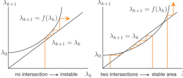
Fig. 7 Graphic assessment of system stability.

the stability of the system. This approach is briefly summarized as follows. First, we introduce time scaleT that represents the time scale that matches the human response rate (for using the communication service). Next, we consider discrete time intervals that are T long. Since the system speed is very high,T is very long for the system but realistic for the customers. Thus, we regard that the system is basi- cally in equilibrium in eachT, and any change in the system maintains the equilibrium (i.e., it is quasi-static).

Based on the above assumption, we represent the input rate including retry traffic at discrete timekasλk. The input rateλk+1 at discrete timek+1 is obtained from sum of the primary traffic rateλ₀ and the retry traffic rate determined by the input rateλkat discrete timek, as

λk+1 =λ₀+ λk/μ

1−λk/μ, (12)

where, the second term on the right hand side denotes retry traﬃc, and at equilibrium, it is proportional to the average number of active customers of M/M/1 [15]. This model corresponds to the high-speed limit of the system and allows us to extract a simple relation between users and the systems as a deterministic model.

We define that the system is stable if the input traﬃc does not diverge, that is, limk→∞λk <∞. Stability can be discussed graphically. In Fig. 7,λk+1 = f(λk) shows (12).

If there are intersections of f(λ_k) and the line with gradient of 1, the system is stable under certain initial conditions. If there is no intersection, the system is instable.

In actual systems, since the speed of the systems is high but finite, the approach takes the diﬀerence from the deterministic model into consideration as fluctuations (Fig. 8).

Then, by choosing an appropriate quantity X(t) that repre- sents the volume of input traﬃc, the temporal evolution of X(t) obeys the following stochastic process,

dX(t)=g₁(X) dt+g₂(X) dW(t), (13) whereg₁(X) denotes the deterministic change obtained from the infinite-speed limit of the system. W(t) is the Wiener process for describing the diﬀerence from the infinite-speed model as fluctuations, andg₂(X) denotes the strength of the fluctuations. Changing the perspective, ifp(x,t) is the probability density function ofX(t), the temporal evolution equation of p(x,t) is expressed as the following Fokker-Planck equation [9],

(7)

Fig. 8 Concept of the quasi-static approach.

∂

∂t p(x,t)= ∂

∂xg₁(x)+ ∂²

∂x²g₂(x)

p(x,t). (14) From the discussion of the relationship between different layers of the hierarchy, we obtain a partial differential equation. The quasi-static approach describes the interaction between layers by using the difference in time scales and sup- pressing the details of the microscopic structure. Hereafter, we reconsider the quasi-static approach from the viewpoint of renormalization.

3. Introduction of a Renormalization Group and Its Application to the Quasi-Static Approach

In the conventional approach to designing networks, we tend to believe that detailed information of state will yield pre- cise control or an exact design. However, in the hierarchical architecture with space/time scale dependency, since the details of the microscopic lower layer cannot be recognized through macroscopic observations, we need to know what kind of quantities can be obtained at the macroscopic higher layer, systematically. Conversely, the quantity obtainable from higher layer is what is essential for describing the relationship between diﬀerent layers. This is because the unob- servable quantities cannot aﬀect the higher layer, and cannot be controlled from the higher layer. In this section, in order to describe the architecture between layers, we introduce the notion of renormalization, apply it to the formulation of the quasi-static approach, and discuss its physical meaning.

3.1 Renormalization Transformation and Renormalization Group

Renormalization was originally developed in the field of quantum electro dynamics in the 1940’s by Tomonaga, Schwinger, and Feynman [16]. Wilson clarified its physical meaning and introduced the renormalization group in the 1970’s [17].

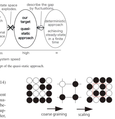
Renormalization transformation is defined as the com- bination of coarse graining transformation and scaling. Let us consider two examples. The first one is the renormalization of diﬀusion (Fig. 4). The temporal evolution of diﬀu- sion corresponds to coarse graining transformation, in this

Fig. 9 Renormalization transformation of infinite 2-dimensional lattice.

case. As a second example, let us consider an infinite Go board. Each grid point is occupied by aGo stone and its color is black with probability p or white with probability 1−p. The problem is how to determine its appearance from afar [18]. First, we adopt the following rule to realize 2×2 subsampling.

• A black stone is set if the 2×2 grid includes three or more black stones.

• A white stone if 2×2 grid includes less than three black stones.

White is slightly favored because white is the more visually prominent than black. This is a coarse graining transformation and yields 1/4 simplification, and then we apply scaling (Fig. 9). These two rules form a renormalization transformation. The probability that the unified grid is black after applying the renormalization transformation just once,R(p), is expressed as

R(p)=p⁴+4p³(1−p). (15) Here, we can findpcsuch thatR(pc)=pcand 0 <pc<1, as

pc= 1+ √ 13

6 ( 0.7676). (16)

This is the critical probability. If p > pc, the board looks black from afar and ifp < pcit looks white. Thus, by using the renormalization transformation, we might be able to describe what can be observed from the macroscopic scale, systematically. The detailed value of p does not aﬀect the macroscopic observation.

(8)

Fig. 10 QTtin the retry traﬃc model of (19).

3.2 Renormalization Transformation of the Arrival Rate Including Retry Traﬃc

Let us introduce the renormalization transformation to the M/M/1 model with retry described in Sect. 2.3. We define the input rateΛ(t;T) at timetas

Λ(t;T)=λ₀+QTt, (17) whereis a positive constant andQTtis a measure of the average number of customers in the system, more specif- ically, QTt is the average within the human-perceptible time periodT immediately before the present timet. So, rateΛ(t;T) is given by the sum of the rateλ₀for the primary traﬃc and the rate for the retry traﬃc, which is proportional to the average number of customers, in the past period.

The following are two concrete examples of the average number of customers,QTt. LetQ(t) be the number of customers in the system at timet, and the first example is

QTt:= 1 T

t⁻ t−T

Q(s) ds. (18)

This model means the rate of retry traﬃc at timetis proportional to the average number of customers in [t−T,T). The second example is

QTt:= 1 T

t⁻

−∞Q(s) e⁻^T¹^(t⁻^s)ds. (19) This model means that the retry from customers ats(<t) oc- curs randomly after exponential time with meanT(Fig. 10).

Regardless of whether we choose (18) or (19) as the defi- nition ofQTt, we can develop a unified discussion. Here- after, unless otherwise noted, the results are valid for both cases.

Ascribing to humans the ability to react immediately corresponds to the limitT →0. From

Tlim→+0QTt=Q(t⁻), (20)

andλ(t) := Λ(t;+0), we have

λ(t)=λ₀+Q(t⁻). (21)

This corresponds to the system model described by the state

transition rate of Fig. 6.

Note that the input rate including the retry traﬃc and the number of customers in the system influence each other.

The variation of the input rate directly affects the number of customers, and conversely the average number of customers affects the input rate through (17). From this discussion, if the human perceptible timeT is changed, the input rate changes through (17) which affects the value ofQ(t). So, to be exact, the number of customers Q(t) must be a quantity that depends on the human perceptible timeT.

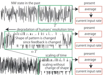
In order to take theT-dependence ofQ(t) into consideration, we introduce the following renormalization transformation. First, we define a coarse graining transformation. Forα ≥ 1, we start to consider the situation that the human time resolution is lowered by 1/α. We call the corresponding transformationKα of the input rate the Kadanoﬀ transformation. The concrete form ofKαfor the average of (18) is

Kα(Λ(t;T))= Λ(t;αT),

=λ₀+ αT

t⁻ t−aT

Q^∗(α,s) ds, (22) and that for (19) is

Kα(Λ(t;T))= Λ(t;αT).

=λ₀+ αT

t⁻

−∞Q^∗(α,s) e⁻^αT¹^(t⁻^s)ds (23) Here,Q^∗(α,t) represents the number of customers according to parameterα, this was changed fromQ(t) by the lowering of the human time resolution. Of course,Q^∗(1,t)=Q(t)^†.

To enable a unified discussion of both cases of (18) and (19), we introduce the following notation for Q^∗(α,t); For (18),

Q^∗_α,β,T

t:= 1 T

t⁻ t−T

Q^∗(α, βs) ds, (24)

and, for (19) Q^∗_α,β,T

t:= 1 T

t⁻

−∞Q^∗(α, βs) e⁻¹^T^(t⁻^s)ds. (25) Using this notation, both (22) and (23) are written in the same form as

Kα(Λ(t;T))=λ₀+ Q^∗_α,1,αT

t. (26)

Next, we introduce the adjustment of time scale by 1/α times, as

Sα(Λ(t;T))=λ₀+

Q^∗_1,α,T/α

t. (27)

Since this is merely a change of scale on the time axis, the form ofQ(t)=Q^∗(1,t) is unchanged.

By combining the above two transformations [3], we

†According to this notation,Q(t⁻), which appears in (20) and (21), is expressed asQ^∗(+0,t⁻), if we assumeα <1.

(9)

Fig. 11 Renormalization transformation for the model of (18).

define the renormalization transformationRαas,

Rα:=Sα◦ Kα. (28) The concrete form of the renormalization transformation of the input rateΛ(t;T) is denoted as

Rα(Λ(t;T))={Sα◦ Kα}(Λ(t;T))

=λ₀+ Q^∗_α,α,T

t. (29)

Figure 11 explains the procedures of the renormalization transformation for the case that the average number of customers is chosen as (18). Incidentally, the renormalization transformations form a semi-group,

R1(Λ(t;T))= Λ(t;T), (30) {Rα◦ Rβ}(Λ(t;T))=Rαβ(Λ(t;T)), (31) {Rαβ◦ Rγ}(Λ(t;T))={Rα◦ Rβγ}(Λ(t;T)), (32) that is called as the renormalization group. Hereafter we denoteΛα(t;T) :=Rα(Λ(t;T)) for brevity.

3.3 Renormalization Group Equation of Arrival Rate and the Quasi-Static Approach

Since we cannot know the concrete form of Q^∗(α,t) for a generalα, we cannot determine the average

Q^∗_α,α,T

tin (29) and therefore the input rateΛα(t;T) cannot be determined for a generalα. Here, we consider a special case of the renormalization transformation withα1, and investigate Λα(t;T). This case means that the speed of the system is much higher than that of humans as expressed by perceptible time scaleT. We assume the following renormalization group equation,

∂

∂αΛα(t;T)=0. (33)

The physical meaning of this equation is that even if we lower the human time resolution further, no new behavior emerges.

To see explicitly the eﬀects of diﬀerentiation with respect to α, we change the expression of (29) into a form that simplifies investigation. SinceSαis merely a change of scale on the time axis, it is an identity transformation, as a transformation ofΛ(t;T). Therefore, (27) is expressed as

Sα(Λ(t;T))=λ₀+

Q^∗_1,α,T/α

t

=λ₀+ Q^∗_1,1,T

t

= Λ(t;T). (34)

From (33) and (34), we have

∂

∂αΛα(t;T)= ∂

∂αKα(Λ(t;T))

= ∂

∂α

Q^∗_α,1,αT

t

=0. (35)

This means the average Q^∗_α,α,T

t is unchanged even if T becomes longer, and so we can recognize that the average remains in a steady state.

4. Reduction of Dynamics and Quasi-Static Approach In this section, we introduce the adiabatic approximation and show that it leads to the same result obtained by the renormalization. In addition, we discuss the description of non-adiabatic eﬀects and relationship to the quasi-static approach.

4.1 Adiabatic Approximation and Renormalization Group Equation

Adiabatic approximation was originally used in solid state physics, and is based on the fact that the nuclei of mole- cules and solids move much more slowly than electrons. It approximates the state of electrons by assuming that the nu- cleus is stationary. This approach is applicable to systems consisting of very slow and very fast components.

First, we introduce the adiabatic approximation taken from [19]. Let us consider the following system. The system moves to relaxed stateq(t)=0 if no external force ex- ists, and the strength of the relaxation is proportional to the diﬀerenceq(t) from equilibrium 0. When we apply external forceF(t) to the system, we have

d

dtq(t)=−γq(t)+F(t), (36)

whereq(t) is the portion of the input rate that corresponds to retries,

q(t) := Λα(t;s)−λ₀, (37)

andγ >0. The solution of (36) is given as q(t)=

t 0

e⁻^γ(t⁻^s)F(s) ds. (38)

(10)

We can recognize thatq(t) is the response to inputF(t). In general,q(t) depends on not only F(t) at the present mo- ment but also the external force in the past. Ifq(t) changes much more rapidly thanF(t), we can recognize that only the external force at the present moment influencesq(t). For example, let the time constant of F(t) be 1/δ, and we set F(t) = ae⁻^δt wherea is a constant. Substituting this into (38) and executing the integration, we obtain

q(t)= a γ−δ

e⁻^δt−e⁻^γt

. (39)

Here we use the assumption that the change ofq(t) is much faster than that ofF(t), that isγδ, so

q(t) a

γe⁻^δt≡ 1

γF(t). (40)

This situation means the time constant of the system, 1/γ, is much smaller than the time constant of the external force, 1/δ.

This treatment is called adiabatic approximation. Note that the approximation (40) is also obtained from (36) by setting dq(t)/dt=0.

Next, we consider the relationship between the adiabatic approximation and the renormalization group. Let us start from (29),

Λα(t;T)=λ₀+ Q^∗_α,α,T

t. (41)

The adiabatic approximation gives Λα(t;T)=λ₀+1

γF(t). (42)

By comparing this with (41), we have the slow external force as

F(t)=γ Q^∗_α,α,T

t. (43)

Thus, (36) becomes d

dtq(t)=γ

−q(t)+ Q^∗_α,α,T

t

, (44)

and, from the adiabatic approximation of (44), we have q(t)=

Q^∗_α,α,T

t. (45)

In addition, by applying the adiabatic approximation dq(t)/dt=0 again, we have

d dt

Q^∗_α,α,T

t=0. (46)

The physical meaning of this result is that the average number of customers is independent of time. In other words, we can regard the average

Q^∗_α,α,T

tis in a steady state, the same as (35) in renormalization.

4.2 Perturbation Expansion of Non-Adiabatic Eﬀects and Understanding of the Quasi-Static Approach

Both the renormalization group Eq. (33) and the adiabatic

approximation correspond to the limit of the situation that the system speed is significantly higher than that of the customers, and both give the same result. However, as shown in Fig. 8, our original goal is a system that has high but finite speed. Therefore, we should also take non-adiabatic eﬀects into consideration.

We introduce the parameterδthat represents the users’

speed and consider the slow variable Q^∗_α,α,T

tand the fast variableq(t), as follows.

⎧⎪⎪⎪⎪⎪⎨

⎪⎪⎪⎪⎪

⎩ d dt

Q^∗_α,α,T

t=δG

Q^∗_α,α,T

t,q , d

dtq(t)=−γq(t)+γ Q^∗_α,α,T

t,

(47)

where G(·,·) is an unknown function. The human perceptible time scale is extremely long compared with that of the system. So, we introduce the smallness parameter η :=δ/γ =1/T 1, whereηrepresent the ratio of users’

speed to the system speed. Next, we set the time constant of the system as 1/γ=1. This procedure means the change of the unit of time or the replace oft→(t/γ), and we have

⎧⎪⎪⎪⎪⎪⎨

⎪⎪⎪⎪⎪

⎩ d dt

Q^∗_α,α,T

t=ηG

Q^∗_α,α,T

t,q , d

dtq(t)=−q(t)+ Q^∗_α,α,T

t.

(48)

We need to investigate the asymptotic behaviors, for t →

∞, of the system that include adiabatic and non-adiabatic eﬀects. To this end, we take the perturbative approach with respect to the power of the smallness parameter in order to describe the small non-adiabatic eﬀects around the adiabatic approximation.

First, we consider the lowest order of the perturbation.

We introduce the notation of the slow variable in (45) as Q^∗t:=

Q^∗_α,α,T

t, (49)

for brevity. The adiabatic approximation is then expressed as ⎧⎪⎪⎪⎨

⎪⎪⎪⎩

qad(t)=Q^∗t, d

dtQ^∗t=ηG

Q^∗t,q_ad(t). (50) In order to realize the higher order correction of non- adiabatic eﬀects around the adiabatic approximation, we take the following approach [20]–[22].

• Because the neutral stability ofQ^∗t triggers the emergence of a secular term (that includes the factor (ηt)) in perturbation, perturbation expansion cannot be applied to Q^∗t. However, since (dQ^∗t/dt) is a small variable, we can apply perturbation expansion to it.

• The perturbation expansion of q(t) around q_ad(t) is of course possible.

• q(t) is dependent on time only throughQ^∗t.

• As long as the perturbation is small (that is, Q^∗t is a slow variable), there is an invariant manifold to which the

(11)

trajectory ofq(t) approaches fort→ ∞.

This treatment was introduced to eliminate the secular term from the perturbation expansion based on the renormalization group [20], and to reduce the degrees of freedom in evaluation equations that describe system dynamics [21]. In any case, the existence of the invariant manifold is critically important in successfully applying this treatment, and it is, exactly,renormalizability[22].

According to the above discussion, let us consider the following perturbation expansions

⎧⎪⎪⎪⎨

⎪⎪⎪⎩

q(t)=q0(t)+ηq₁(t)+η²q2(t)+η³q3(t)+· · ·, d

dtQ^∗t=v₀(t)+ηv₁(t)+η²v₂(t)+η³v₃(t)+· · ·. (51) Based on the adiabatic approximation (50),

q₀(t)=q_ad(t), and v₀(t)=0. (52) By using the expansion ofq(t), the higher-order correction of non-adiabatic eﬀects in

dQ^∗t/dt

is expressed as d

dtQ^∗t=ηG

Q^∗t,q₀(t)+ηq₁(t)+O(η²)

=ηGQ^∗t, Q^∗t

+η²

∂GQ^∗t,q

∂q

q=q₀

q1(t)

+O(η³). (53)

Therefore, we have

v₁(t)=GQ^∗t, Q^∗t

, (54)

v₂(t)=

∂GQ^∗t,q

∂q

q=q0

q1(t). (55)

Next, we consider the higher-order correction of non- adiabatic eﬀects in q(t). Because the time dependency of q(t) occurs only throughQ^∗t, we representq(t)=q(Q˜ ^∗t) for convenience. From (44), we have

dQ^∗t

dt

d ˜q(Q^∗t) dQ^∗t

=−q(t)+Q^∗t. (56) By expanding this as,

(ηv₁(t)+O(η²)) d dQ^∗t

( ˜q0(Q^∗t)+O(η))

=−(q0(t)+ηq₁(t)+O(η²))+Q^∗t, (57) and by extracting the terms of the order ofη, we have

v₁(t)d ˜q0(Q^∗t) dQ^∗t

=−q1(t). (58) Thus, we have

q₁(t)=−GQ^∗t, Q^∗t

d ˜q₀(Q^∗t) dQ^∗t

=−G

Q^∗t, Q^∗t

. (59)

We can summarize the results as

⎧⎪⎪⎪⎪⎪⎪⎪⎪

⎪⎨⎪⎪⎪⎪⎪

⎪⎪⎪⎪⎩

d

dtQ^∗t=ηGQ^∗t, Q^∗t

+η²

∂G

Q^∗t,q

∂q

q=q₀

q1(t)+O(η³), q(t)=Q^∗t−ηGQ^∗t, Q^∗t

+O(η²).

(60) From (60), there is no term of the order ofη⁰in (dq(t)/dt).

This means the variation ofQ^∗tandq(t) are not observed at the time scale ofT⁰=1, but it does appear at the time scale ofT¹. This result corresponds to the quasi-static approach;

the system is in the equilibrium state when observed at the time scale ofT, and the state changes very slowly keeping the equilibrium state. Therefore, by introducing the time step unit ofT, we define

λk:= Λα(kT,T), k=1,2, . . . , (61) and the temporal evolution of (61) can be described by (12).

4.3 Temporal Evolution Equation of the Number of Arriv- ing Customers Including Retries

In this subsection, we adopt the average number of customers in the system as (18) and define the actual number of customers arriving during [t−T,t⁻] asX(t,T)^†. IfT → ∞, that is the limit of higher system speed, the observed input rate is equivalent to the input rateX(t,T)/T = Λα(t;T).

However, for a finite T,X(t,T)/T Λα(t;T), in general.

When we discuss the diﬀerence from the high speed limit as shown in Fig. 8, we should describeX(t,T)/T rather than Λα(t;T).

The variation ofX(t,T)/T occurs very slowly but can be observed at the human perceivable scale. This observation is equivalent to fast forwarding a video.

Next we determine the details of the unknown function G(·,·) in (60), by using model-specific characteristics of large-scale M/M/1. The infinitesimal variation ofX(t,T) is defined as

dX(t,T) :=X(t+dt,T)−X(t,T)

=X(t+dt,dt)−X(t−T+dt,dt). (62) We assume that the timing of retry traﬃc input is fully ran- domized and it follows a Poisson process. In addition, the large-scale system targeted has a large value of primary traffic rate λ₀, and thus the Poisson distribution is suﬃciently close to the normal distribution. Therefore, the number of arriving customers can be expressed, by using the Wiener process, as

X(t+dt,dt)= Λα(t,T) dt+

Λα(t,T) dW(t)

†Of course, we can adopt (19) alternatively.

(12)

=

λ₀+ X(t,T)/(μT) 1−X(t,T)/(μT)

dt +

λ₀+ X(t,T)/(μT)

1−X(t,T)/(μT)dW(t), (63) X(t−s+dt,dt)= X(t,T)

T dt+

X(t,T)

T dW(t). (64) Thus the infinitesimal variation ofX(t;T) is obtained as

dX(t,T)=

λ₀−X(t,T)

T + X(t,T)/(μT) 1−X(t,T)/(μT)

dt +

λ₀+X(t,T)

T + X(t,T)/(μT) 1−X(t,T)/(μT)dW(t).

(65) In the form of Langevin equation, (65) can be expressed as

dX(t,T)

dt =

λ₀−X(t,T)

T + X(t,T)/(μT) 1−X(t,T)/(μT)

+

λ₀+X(t,T)

T + X(t,T)/(μT) 1−X(t,T)/(μT)ξ(t),

(66) whereξ(t) is the white Gaussian noise that satisfies E[ξ(t)]= 0 and E[ξ(t)ξ(s)] = δ(t−s), and ξ(t) obeys the standard normal distribution. This result corresponds to (13) and we can also express the result in the form of (14) as

∂

∂t pT(x,t)

= ∂

∂x

λ₀−X(t,T)

T + X(t,T)/(μT) 1−X(t,T)/(μT)

pT(x,t) + ∂²

∂x²

λ₀+X(t,T)

T + X(t,T)/(μT)

1−X(t,T)/(μT)pT(x,t), (67) wherepT(x,t) is the probability density function ofX(t,T).

The validity of (65) and (67) was verified by comparison against simulation results in [23].

5. Conclusions

In this paper, we have discussed the design of a network architecture that adopts the approach of reproducing the stability and order of nature. Our guiding principle is hierarchy with time scale dependency, and it includes the local-action theory and the renormalization group. We demonstrated the importance of the renormalization group in hierarchical design by using an example of interaction between customers and a system. The form of the temporal evolution Eq. (67) describes the phenomena of pT(x,t) observed at the hu- man perceptible macro-scale, and eﬀects from more finely- granular structures reflecting state transition of the system

are reduced and represented as the value of the coeﬃcient of (67). This is an example of hierarchical structure shown in Sect. 2.3. In addition, we clarified the physical interpreta- tion of the quasi-static approach.

Acknowledgment

This research is supported by a Grant-in-Aid for Scientific Research (B) No. 21300027 (2009–2011) from the Japan Society for the Promotion of Science.

References

[1] M. Aida, C. Takano, and Y. Sakumoto, “Challenges to new network architectures based on hierarchical structure of time scales,”

J. IEICE, vol.94, no.5, pp.401–406, May 2011.

[2] C. Takano and M. Aida, “Autonomous decentralized flow control mechanism based on diﬀusion phenomenon as guiding principle:

Inspired from local-action theory,” J. IEICE, vol.91, no.10, pp.875–

880, Oct. 2008.

[3] Y. Oono, H. Tasaki, and K. Higashijima, “Expanding horizon of renormalization theory,” Mathematical Sciences, Saiensu-sha, Pub- lishers (in Japanese), vol.35, no.4, pp.5–12, 1997.

[4] M. Aida and C. Takano, “Principle of autonomous decentralized flow control and layered structure of network control with respect to time scales,” Supplement of the ISADS 2003 Conference Fast Abstracts, pp.3–4, 2003.

[5] G. Neglia and G. Reina, “Evaluating activator-inhibitor mechanisms for sensors coordination,” IEEE/ACM BIONETICS 2007, pp.129–

133, Budapest, Hungary, Dec. 2007.

[6] N. Wakamiya, K. Hyodo, and M. Murata, “Reaction-diﬀusion based topology self-organization for periodic data gathering in wireless sensor networks,” Second IEEE International Conference on Self- Adaptive and Self-Organizing Systems, pp.351–360, Venice, Italy, Oct. 2008.

[7] K. Leibnitz and M. Murata, “Attractor selection and perturbation for robust networks in fluctuating environments,” IEEE Network, vol.14, no.3, pp.14–18, May/June 2010.

[8] C. Constantinou and A. Stepanenko, “Network protocol scalability via a topological Kadanoﬀtransformation,” 6th International Sym- posium on Modeling and Optimization (WiOPT 2008), pp.560–563, April 2008.

[9] N.G. van Kampen, Stochastic Processes in Physics and Chemistry, 3rd ed., North Holland, 2007.

[10] C. Takano and M. Aida, “Diﬀusion-type autonomous decentralized flow control for end-to-end flow in high-speed networks,” IEICE Trans. Commun., vol.E88-B, no.4, pp.1559–1567, April 2005.

[11] M. Uchida, K. Ohnishi, K. Ichikawa, M. Tsuru, and Y. Oie, “Dy- namic and decentralized storage load balancing with analogy to thermal diﬀusion for P2P file sharing,” IEICE Trans. Commun., vol.E93-B, no.3, pp.525–535, March 2010.

[12] C. Takano, M. Aida, M. Murata, and M. Imase, “New framework of back diﬀusion-based autonomous decentralized control and its application to clustering scheme,” IEEE Globecom 2010 Workshop on the Network of the Future (FutureNet III), 2010.

[13] C. Takano, M. Aida, M. Murata, and M. Imase, “Autonomous decentralized mechanism of structure formation adapting to network conditions,” 11th IEEE/IPSJ International Symposium on Applica- tions and the Internet (SAINT 2011) Workshops (HEUNET 2011), Munich, Germany, July 2011.

[14] T. Kubo, T. Hasegawa, and T. Hasegawa, “Mathematically designing a local interaction algorithm for autonomous and distributed systems,” 10th International Symposium on Autonomous Decentralized Systems (ISADS 2011), 194–203, March 2011.

[15] M. Aida, C. Takano, M. Murata, and M. Imase, “A study of control