A test for high-dimensional covariance matrices via the extended cross-data-matrix methodology (Statistical Inference and Modelling)

全文

(1)11. A test for high‐dimensional covariance matrices via the extended cross‐data‐matrix methodology Kohei Endo. Graduate School of Pure and Applied Sciences University of Tsukuba Kazuyoshi Yata Institute of Mathematics. University of Tsukuba Makoto Aoshima Institute of Mathematics. University of Tsukuba. Abstract. In this paper, we consider two‐sample tests for covariance matrices in high‐dimensional settings. We introduce the extended cross‐data‐matrix (ECDM) methodology. We con‐ struct test statistics by using the ECDM methodology. We show that the ECDM test statistics have the consistency property and the asymptotic normality in high‐dimensional settings. We propose a new test procedure based on the ECDM test statistics and evaluate its asymptotic size and power from theoretical and numerical aspects.. Keywords and phrases: Asymptotic normality; ECDM; HDLSS; Large p , small. 1. n. Introduction. High‐dimension, low‐sample‐size (HDLSS) data situations occur in many areas of modern science such as genetic microarrays, medical imaging, text recognition, finance, chemometrics, and so on. In recent years, substantial work has been done on HDLSS asymptotic theory in which the sample size n is fixed or narrow\infty while n/parrow 0 as the data dimension parrow\infty.. Hall et al. [6] and Yata and Aoshima [11] explored several types of geometric representa‐ tions of HDLSS data. Yata and Aoshima [11] developed the noise‐reduction methodology and gave consistent estimators of both the eigenvalues and eigenvectors together with principal. component (PC) scores in the HDLSS context. The HDLSS asymptotic theory was created.

(2) 2 under the assumption that either the population distribution is Gaussian or random vari‐ ables in a certain sphered data matrix have the \rho‐mixing dependency. However, Yata and. Aoshima [10] developed the HDLSS asymptotic theory without such the assumptions. More‐ over, they created a new principal component analysis (PCA) called the cross‐data‐matrix (CDM) methodology that is applicable to constructing an unbiased estimator in HDLSS non‐ parametric settings. Aoshima and Yata [2] developed a variety of inference for HDLSS data such as given‐bandwidth confidence regions, two‐sample tests, tests of the equality of two covariance matrices, classification, variable selection, regression, tests of the correlation co‐ efficients and so on, and also discussed the sample size determination to ensure prespecified. accuracy for each inference. Yata and Aoshima [12] improved the test of the correlation co‐ efficients by using the extended cross‐data‐matrix (ECDM) methodology that is an extension of the CDM method. One of the advantages of the ECDM methodoıogy is to produce an unbiased estimator having small asymptotic variance at a low computational cost. In this paper, we consider two‐sample tests for high‐dimensional covariance matrices.. Let. x_{h1},. x_{hn_{h}}. be independent and identically distributed (i.i. d. ) samples of a p‐‐variate. random variable from populations \pi h(h=1,2) . We assume n_{1}/n_{2}arrow\theta\in(0, \infty) and nh<p for h=1,2 . We assume that x_{hj} has an unknown mean vector \mu_{h} and unknown covariance matrix \Sigma_{h}(\geq O) for h=1,2 . We consider a test problem as follows: H_{0}:\Sigma_{1}=\Sigma_{2}. vs.. H_{1} : \Sigma_{1}\neq\Sigma_{2} .. (1). The test problem has been studied in the conventional low‐dimensional settings. In particular,. the likelihood ratio test (LRT) is commonly used and enjoys certain optimality under regular‐ ity conditions, see Anderson [1]. However, in the high‐dimensional settings, the conventional test procedures such as the LRT perform poorly or are not even defined since the sample covariance matrix S , the simplest estimator of the population covariance matrix \Sigma , performs. poorly. Li and Chen [8] gave a test statistic based on U‐statistics for high‐dimensional data. However, it requires high computational cost. Srivastava et al. [9] improved the statistic in terms of computational cost. In this paper, we shall produce statistics by the ECDM method and propose a new test procedure for (1). The rest of the paper is organized as follows. In Section 2, we state assumptions required in the construction of a test procedure for (1). In Section 3, we introduce the ECDM method‐ ology. In Section 4, we produce test statistics for (1) by using the ECDM methodology. We show that the ECDM test statistics have the consistency property and the asymptotic nor‐ mality in high‐dimensional settings. We propose a new test procedure based on the ECDM test statistics and evaluate its asymptotic size and power theoretically. Finally, in Section 5, we give simulation studies to check the performance of the proposed test procedure.. 2. Assumptions In this section, we introduce the basic assumptions for the test of hypotheses (1). The. eigen‐decomposition of \Sigma_{h} is given by. \Sigma_{h}=H_{h}\Lambda_{h}H_{h}^{T} , where \Lambda_{h}=diag(\lambda_{h1}, \ldots, \lambda_{hp}) is a.

(3) 3 diagonal matrix of eigenvalues, \lambda_{h1}\geq corresponding eigenvectors. Now, we assume the following model:. \geq\lambda_{hp}\geq 0 , and H_{h} is an orthogonal matrix of the. x_{hj}=\Gamma_{h}w_{hj}+\mu_{h} ,. for h=1,2,. is a p\cross q_{h} matrix for some q_{h}>0 such that \Gamma_{h}\Gamma_{h}^{T}=\Sigma_{h} , and n_{h} , are i.i. d . random vectors having E(w_{hj})=0 and j=1, . Here, denotes the identity matrix of dimension q_{h} . Let Var(w_{hrj}^{2})=M_{hr}, Var(w_{hj})=I_{q_{h}} I_{q_{h}} r=1, q_{h};h=1,2 . We assume that \lim\sup_{parrow\infty}M_{hr}<\infty for all h, r . Similar to Aoshima. \Gamma_{h}=(\gamma_{h1}, \ldots, \gamma_{hq_{h} ) w_{hj}=(w_{h1j}, \ldots, w_{hq_{h}j})^{T},. where. and Yata [3] and Bai and Saranadasa [4], we assume that. E(w_{hrj}^{2}w_{hsj}^{2})=E(w_{hrj}^{2})E(w_{hsj}^{2})=1. (A‐i). and E(w_{hrj}w_{hsj}w_{htj}w_{huj})=0 for all r\neq s,. t,. u.. We assume the following assumption instead of (A‐i) as necessary:. (A‐ii). E(w_{hr_{1}j}^{\alpha_{1} w_{hr_{2}j}^{\alpha_{2} \cdots w_{hr_{v}j} ^{\alpha_{v} )=E(w_{hr_{1}j}^{\alpha_{1} )E(w_{hr_{2}j}^{\alpha_{2} )\cdots E(w_ {hr_{v}j}^{\alpha_{v} ). [1, q_{h}] and \alpha_{i}\in[1,4], i=1,. v. , where v\leq 8 and. for all r_{1}\neq r_{2}\neq. \neq r_{v}\in. \sum_{\iota={\imath} ^{v}\alpha_{i}\leq 8.. See Chen and Qin [5] about (A‐ii). Note that (A‐ii) implies (A‐i). Note that (A‐ii) is naturally. satisfied when. ( A‐iii). x_{hj}. is Gaussian. We assume the following assumption for \Sigma_{h} as necessary:. \frac{tr(\Sigma_{h}^{4}){tr(\Sigma_{h}^{2})^{2}ar ow0. Note that. as. parrow\infty. for h=1,2.. tr(\Sigma_{h}^{4})/tr(\Sigma_{h}^{2})^{2}arrow 0. a\mathfrak{Z}parrow\infty for. as parrow\infty for h=1,2 ” is equivalent to \lambda_{h1}/tr(\Sigma_{h}^{2})^{ \imath}/2}arrow 0 h=1,2 ”. Let m= \min\{p, n_{1}, n_{2}\} and \triangle=||\Sigma_{1}-\Sigma_{2}||_{F}^{2}=tr\{(\Sigma_{1}-\Sigma_{2})^{2}\}.. We assume one of the following two assumptions as necessary:. (A‐iv) (A‐v). 3. for \frac{tr(\Sigma_{h}^{2}) {n_{h}\triangle}ar ow0 as 1 i_{M}\sup_{ar ow\infty}\{\frac{n_{h}\triangle}{tr(\Sigma_{h}^{2}) \}<\infty for. h=1,2 ;. marrow\infty. h=1,2.. ECDM methodology. The ECDM methodology was developed by Yata and Aoshima [12, 13] as an extension of the CDM method due to Yata and Aoshima [10]. Throughout this section, we omit the subscript with regard to the population. Let n_{(1)}=\lceil n/2\rceil and n(2)=n-n_{(1)} , where \lceil x\rceil denotes the smallest integer \geq x . Let. V_{n(1)(k)}=\{ begin{ar ay}{l} \{ lfo rk/2\rflo r-n_{(1)}+1,\lfo rk/2\rflo r\} if\lfo rk/2\rflo r \geqn({\imath}), \{1,\lfo rk/2\rflo r\} cup\{ lfo rk/2\rflo r+n_{(2)}+1,n\} otherwise; \end{ar ay} V_{n(2)(k)}=\{ begin{ar ay}{l} \{ lfo rk/2\rflo r+1,\lfo rk/2\rflo r+n_{(2)}\ if\lfo rk/2\rflo r\leq n_{(1)}, \{1,\lfo rk/2\rflo r-n_{(1)}\ cup\{ lfo rk/2\rflo r+1,n\} otherwise \end{ar ay}.

(4) 4 for k=3,. 2n-1 ,. where \lf o r x\rflo r denotes the largest integer \leq x . Let \# S denote the number. of elements in a set S .. Note that. \# V_{n(l)(k)}=n_{(l)}, l=1,2, V_{n(1)(k)}\cap V_{n(2)(k)}=\emptyset and 2n-1 . Also, note that i\in V_{n(1)(i+j)} and. n } for k=3, V_{n(1)(k)}\cup V_{n(2)(k)}= {ı, j\in V_{n(2)(i+j)} for i<j(\leq n) . Let. \overline{x}_{n(1)(k)}=n_{(1)}^{-1}\sum_{j\in V_{n(1)(k)} x_{j} for k=3,. 2n-1 .. \overline{x}_{n(2)(k)}=n_{(2)}^{-1}\sum_{j\in V_{n(2)(k)} x_{j}. and. Then, Yata and Aoshima [12] gave an estimator of tr(\Sigma^{2}) by. W_{n}= \frac{2u_{n} {n(n-1)}\sum_{i<j}^{n}\{(x_{i}-\overline{x}_{n(1)(i+j)}) ^{T}(x_{j}-\overline{x}_{n(2)(i+j)})\}^{2} where. u_{n}=n_{(1)}n_{(2)}/\{(n_{(1)}-1)(n_{(2)} -{\imath})\} .. Note that. E(W_{n})=tr(\Sigma^{2}) .. ,. Let. Aoshima and Yata [3] and Yata and Aoshima [13] gave the following result. Theorem 3.1 ([3, 13]). Assume (A‐i). Then, it holds that as. (2). m_{0}= \min\{p, n\}.. m_{0}arrow\infty. Var( \frac{W_{n} {tr(\Sigma^{2}) =(\frac{4}{n^{2} +\frac{8tr(\Sigma^{4})+ 4\sum_{r- 1}^{q}(M_{r}-2)(\gamma_{r}^{T}\Sigma\gamma_{r})^{2} {tr(\Sigma^{2}) ^{2}n})\{1+o(1)\}. Remark 1. When x_{j} is Gaussian, it holds that as Var. 4. m_{0}arrow\infty. ( \frac{W_{n} {tr(\Sigma^{2}) =(\frac{4}{n^{2} +\frac{8tr(\Sigma^{4}) {tr(\Sigma^{2})^{2}n})\{1+o(1)\}.. Two‐sample tests for covariance matrices. In this section, we consider two‐sample tests for covariance matrices using the ECDM methodology. Let us consider the following hypotheses which are equivalent to (1): H_{0}:\triangle=0. vs.. H_{1}. :. \triangle>0.. Note that \Delta=tr(\Sigma_{1}^{2})+tr(\Sigma_{2}^{2})-2tr(\Sigma_{1}\Sigma_{2}) . Li and Chen [8] proposed a test statistic as follows:. U=A_{n_{1}}+A_{n_{2}}-2tr(S_{1n_{1}}S_{2n}2). ,.

(5) 5 where S_{hn_{h}} is the sample covariance matrix having E(S_{hn_{h}})=\Sigma_{h} and. A_{n_{h} = \frac{1}{n_{h}(n_{h}-1)}\sum_{j\neq k}^{n_{h} (x_{hj}^{T}x_{hk})^{2} -\frac{2}{n_{h}(n_{h}-1)(n_{h}-2)}\sum_{j\neq k\neq l}^{n_{h} x_{hk}^{T}x_{hj}x_ {hj}^{T}x_{hl} + \frac{1}{n_{h}(n_{h}-1)(n_{h}-2)(n_{h}-3)}\sum_{j\neq k\neq l\neq l'}^{n_{h} x_{hj}^{T}x_{hk}x_{hl}^{T}x_{hl'}. Under (A‐ii), ( A‐iii) and some regularity conditions, they showed the following asymptotic result:. \frac{U-\triangle}{2tr(\Sigma_{1}^{2})/n_{1}+2tr(\Sigma_{2}^{2})/n_{2} \Rightar ow N(0,1) as. marrow\infty. .. (3). Here, "\Rightarrow denotes the convergence in distribution and N(0,1) denotes a random variable distributed as the standard normal distribution. However, the computational cost of A_{n_{h}} is of the order, O(pn_{h}^{4}) , which is inappropriate for practical use. On the other hand, Srivastava. et al. [9] modified A_{n_{h}} as. \frac{(n_{h}-1)(n_{h}-2)tr(M_{h}^{2})-n_{h}(n_{h}-1)tr(D_{h}^{2})+tr(D_{h}) ^{2} {n_{h}(n_{h}-1)(n_{h}-2)(n_{h}-3)} where. Y_{h}=(y_{h1}, \ldots, y_{hn_{h}}),. y_{hj}=x_{hj}-\overline{x}_{h},j=1,. Y_{h}^{T}Y_{h}, D_{h}=diag(y_{h1}^{T}y_{h1}, \ldots, y_{hn_{h}}^{T}y_{hn_{h}}) , of the order, O(pn_{h}^{2}) . Let. n_{h},. ( =A_{n_{h}}^{*} , say),. \overline{x}_{h}=n_{h}^{-1}\sum_{j=1}^{n_{h} x_{hj},. for h=1,2 . The computational cost of. M_{h}=. A_{n_{h} ^{*} is. \sigma U=2(\frac{1}{n_{1}-1}+\frac{1}{n_{2}-1})\frac{(n_{1}-1)tr(\Sigma_{1} ^{2})+(n_{2}-1)tr(\Sigma_{2}^{2})}{n_{1}+n_{2}-2} and. \hat{\sigma}_{U}=2. ( \frac{1}{n_{1}-} \frac{1}{n_{2}-1})\frac{(n_{1}-1)A_{n_{1} ^{*}+(n_{2}-1)A_{n2}^{*} {n_{1}+ n_{2}-2}. ı. +. Then, they gave a test procedure for (1) by rejecting where. z_{\alpha}. H_{0} \Leftrightar ow\frac{U}{\hat{\sigma}_{U} >z_{\alpha} ,. (4). is a constant such that P\{N(0,1)>z_{\alpha}\}=\alpha . Then, under (A‐ii) and ( A‐iii), it. holds that as. marrow\infty. Size. Also, we have the following result.. =\alpha+o(1) ..

(6) 6 Theorem 4.1. Assume (A‐ii) and ( A ‐iii). The test by (4) has that as Power. marrow\infty. = \Phi(\frac{\triangle}{\sigma_{U} -z_{\alpha})+o(1) ,. (5). where \Phi(\cdot) denotes the c.d.f. of N(0,1) . In this paper, we give a more powerful test statistic compared with. 4.1. U.. A test statistic based on the ECDM methodology Now, by using the ECDM methodology, we estimate. \triangle. by. T=W_{n_{1}}+W_{n_{2}}-2tr(S_{1n_{1}}S_{2n_{2}}). ,. where W_{n_{h}}s are given by (2). Note that E(T)=\triangle . Also, note that the computational cost of W_{n_{h}} is of the order, O(pn_{h}^{2}) . Let. \sigma^{2}=\sum_{h=1}^{2}(\frac{4}{n_{h}^{2} tr(\Sigma_{h}^{2})^{2}+\frac{8} {n_{h} tr\{(\Sigma_{h}^{2}-\Sigma_{1}\Sigma_{2})^{2}\}+\frac{4}{n_{h} \sum_{r=1} ^{q_{h} (M_{hr}-2)\{\gam a_{hr}^{T}(\Sigma_{1}-\Sigma_{2})\gam a_{hr}\}^{2}) + \frac{8}{n_{1}n_{2} tr(\Sigma_{1}\Sigma_{2})^{2}.. Then, we have the foılowing result.. Lemma 4.1. Assume (A‐i). It holds that as. marrow\infty. Var(T)=\sigma^{2}\{1+o(1)\}. From Lemma 4.1 we have the following result.. Theorem 4.2. Assume (A‐i) and (A‐iv). It holds that as. \frac{T}{\Delta}=1+o_{P}(1). marrow\infty. .. Next, we consider the case when (A‐iv) is not met. Let. \sigma_{T}^{2}=\frac{4}{n_{1}^{2} tr(\Sigma_{1}^{2})^{2}+\frac{4}{n_{2}^{2} tr (\Sigma_{2}^{2})^{2}+\frac{8}{n_{1}n_{2} tr(\Sigma_{1}\Sigma_{2})^{2} and. \hat{\sigma}_{T}^{2}=\frac{4}{n_{1}^{2} W_{n_{1} ^{2}+\frac{4}{n_{2}^{2} W_{n_ {2} ^{2}+\frac{8}{n_{1}n_{2} tr(S_{1n1}S_{2n2})^{2} We have the following result..

(7) 7 Lemma 4.2. Assume (A‐i), ( A ‐iii) and (A‐v). It holds that as. marrow\infty. \sigma^{2}=\sigma_{T}^{2}\{1+o(1)\}. Note that as. marrow\infty. \frac{\hat{\sigma}_{T}^{2} {\sigma_{T}^{2} =1+O_{P(1)} under (A‐i). From Lemma 4.2 we have the following result.. Theorem 4.3. Assume (A‐ii), ( A ‐iii) and (A‐v). It holds that as. \frac{T-\triangle}{\hat{\sigma}_{T} =\frac{T-\triangle}{\sigma_{T} +o_{P}(1) \Rightar ow N(0,1). marrow\infty. .. Now, we consider a more powerful test statistic. Let. c= \max\{\frac{tr(\Sigma_{1}) {tr(\Sigma_{2}) , \frac{tr(\Sigma_{2}) {tr(\Sigma_{1}) \} Then, under (A‐i), we have that as. and. \hat{c}=\max\{\frac{tr(S_{1n1}) {tr(S_{2n_{2} )}, \frac{tr(S_{2n2}) {tr(S_{1n1}) \}.. marrow\infty. \hat{C}=C+O_{P(1)} .. (6). We propose the following test statistic: T_{*}=\hat{c}T.. Note that T_{*}\geq T w.p.ı. Also, note that as. marrow\infty. T_{*}=T\{1+o_{P}(1)\}. under (A‐i) and H_{0} . Then, from Theorems 4.2 and 4.3, we have the following results. Corollary 4.1. Assume (A‐i) and (A‐iv). It holds that as. \frac{T}{c\triangle}*=1+o_{P}(1). marrow\infty. .. Corollary 4.2. Assume (A‐ii), ( A ‐iii) and (A‐v). It holds that as. \frac{T_{*}/c-\Delta}{\hat{\sigma}_{T} \Rightar ow N(0,1). .. marrow\infty.

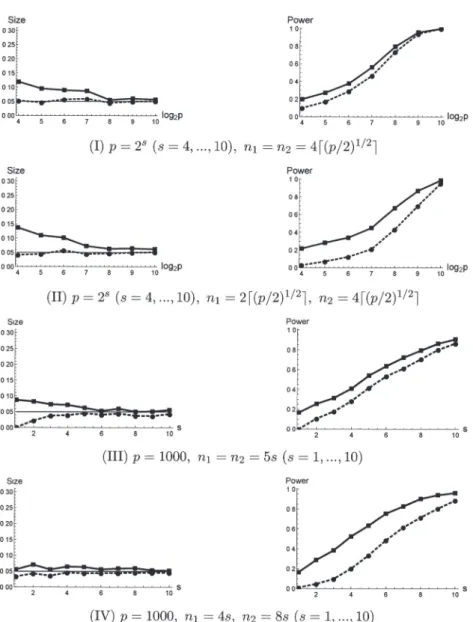
(8) 8 4.2. A more powerful two‐sample test We give a test procedure for (1) by rejecting. H_{0} \Leftrightar ow\frac{T}{\hat{\sigma}_{T} *>z_{\alpha} .. (7). Then, we have the following results.. Theorem 4.4. Assume (A‐ii) and ( A ‐iii). The test by (7) has that as Size=\alpha+o(1). and. Power. marrow\infty. = \Phi(\frac{\triangle}{\sigma_{T} -z_{\alpha}/c)+o(1). .. Corollary 4.3. Assume (A‐iv) under H_{1} . Assume also (A‐i). Then, the test by (7) has that as. marrow\infty. Power. =1+o(1) .. Remark 2. We consider testing (1) by (7) with. T. instead of. T_{*} .. Then, it has (5) as. marrow\infty.. From Theorems 4.1 and 4.4, when c>1 , the asymptotic power of (7) is greater than that of (4). Thus, we recommend to use the test by (7). 5. Simulation studies In this section, we summarize simulation studies of the findings.. We used computer. simulations to study performances of the test procedures by (4) and (7). Independent pseudo‐ random normal observations were generated from and. \Sigma_{1}=B(0.3^{|i-j|^{1/3}})B ,. \pi_{h}. : N_{p}(0, \Sigma_{h}) for h=1,2 . We set. \alpha=0.05. where. B=diag[\{0.5+1/(p+1)\}^{1/2}, \{0.5+p/(p+1)\}^{1/2}]. As for the alternative hypothesis, we set for p and n_{l}s :. (I). (II) (III) (IV). \Sigma_{2}=1.2B(0.4^{|i-j|^{1/3}})B .. We considered four cases. p=2^{S}(s=4, \ldots, 10), n_{1}=n_{2}=4\lceil(p/2)^{1/2}\rceil ; p=2^{S}(s=4, \ldots, 10), n_{1}=2\lceil(p/2)^{1/2}\rceil, n_{2}=4\lceil(p/2)^{1/2}\rceil ; p=1000, n_{1}=n_{2}=5s(s=1, \ldots, 10) ; p=1000, n_{1}=4s, n_{2}=8s(s=1, \ldots, 10) ..

(9) 9. g_{2}p. 2p. (I) p=2^{S}(s=4, \ldots, 10), n_{1}=n_{2}=4\lceil(p/2)^{1/2}\rceil \ulcorner. g_{2}p. 2p. (II) p=2^{s}(s=4, \ldots, 10), n_{1}=2\lceil(p/2)^{1/2}\rceil, n_{2}=4\lceil(p/2)^{1/2}\rceil. (III) p=1000,. n_{1}=n2=5s. (. s=. ı. 10). (IV) p=1000, n_{1}=4s, n_{2}=8s(s=1, \ldots, 10) Figure 1: The performances of the test procedures by (4) and (7). For each panel, the value of (4) is denoted by the dashed ıine and the value of (7) is denoted by the solid line..

(10) 10 For each case, we checked the performance by 2000 replications. We defined P_{r}=1 (or 0 ) when H_{0} was falsely rejected (or not) for r=1 , 2000, and defined \overline{\alpha}=\sum_{r=1}^{2000}P_{r}/2000 to estimate the size. We also defined P_{r}=1 (or 0 ) when H_{1} was falsely rejected (or not) for r=1 , 2000, and defined 1- \overline{\beta}=1-\sum_{r=1}^{2000}P_{r}/2000 to estimate the power. Note that their standard deviations are less than 0.0ıl. In Figure 1, we plotted \overline{\alpha} (left panel) and 1-\overline{\beta} (right panel) in case of (I) to (IV). We observed that both the test procedures gave preferable performances for the size in (I) to (IV). However, the test procedure by (7) gave better performance compared to (4) with respect to the power. See Section 4.2 for the theoretical reason.. Appendix Proof of Theorem 4.1. Note that tr(\Sigma_{1}^{2})=tr(\Sigma_{2}^{2})\{1+o(1)\} as. parrow\infty. under (A‐v). Also,. note that. \sum_{r=1}^{q_{h} \{ gam a_{hr}^{T}(\Sigma_{1}-\Sigma_{2})\gam a_{hr}\ ^{2} \leq. tr [\{\Sigma_{h}(\Sigma_{1}-\Sigma_{2})\}^{2}]\leq\lambda_{h1}^{2}\triangle= o(tr(\Sigma_{h}^{2})\triangle). (8). under ( A‐iii) for h=1,2 . Then, it holds that \sigma/\sigma U=1+o(1) under ( A‐iii) and (A‐v). Thus, from Theorems 1 and 2 in Li and Chen [8], under (A‐ii), ( A‐iii) and (A‐v), we have that as marrow\infty. P( \frac{U}{\hat{\sigma}_{U} >z_{\alpha})=P(\frac{U-\triangle}{\sigma U} >z_{\alpha}-\frac{\triangle}{\sigma_{U} +o_{P}(1) (\begin{ar y}{l \underline{\triangle}-z_{\alpha} \sigma_{U} \end{ar y}) +o(1) =\Phi. .. On the other hand, from (8), under (A‐ii) and (A‐iv), it holds that Var(U)/\triangle^{2}= o(ı), so. that U/\triangle=1+o_{P}(1) . Then, we have that. P( \frac{U}{\hat{\sigma}_{U} >z_{\alpha})=P(\frac{\triangle}{\sigma_{U} \{1+ o_{P}(1)\}>z_{\alpha})ar ow 1 from the fact that \sigma_{U}/\triangle=o(1) under (A‐iv). Thus, by considering the convergent subse‐ \square quence of \triangle/\sigma_{U} , we can conclude the result. Proof of Lemma 4.1. Assume (A‐i). Recall that. T=W_{n_{1}}+W_{n_{2}}-2tr(S_{1n1}S_{2n_{2}}). and. U=A_{n1}+A_{n2}-2tr(S_{1n_{1}}S_{2n_{2}}) ..

(11) 11 11 Note that E(T)=\Delta . By noting that Cov(W_{n_{1}}, W_{n_{2}})=0 , it holds that. Var (T)=Var(W_{n_{1}})+Var(W_{n_{2}})+4Var (tr (S_{1n_{1}}S_{2n_{2}}) ). -4Cov(W_{n_{{\imath}}}, tr(S_{1n_{1}}S_{2n2}))-4Cov(W_{n_{2}}, tr(S_{1n_{1}} S_{2n_{2}})). .. From Theorem 3.1 and (6.2) in [8], we can claim that Var(W_{n_{h}})=Var(A_{n}h)\{1+o(1)\} as marrow \infty for h=1,2 . Also, we can claim that Cov(W_{n_{h}}, tr(S_{1n_{1}}S_{2n_{2}}))=Cov(A_{n_{h}}, tr(S_{1n_{1}}S_{2n_{2}} ))\{1+ \square o(1)\} for h=1,2 . Then, from (2.5) and (6.ı) in [8], we can conclude the result.. Proof of Theorem 4.2. From (8), under (A‐i) and (A‐iv), it holds that Var(T)/\triangle^{2} that T/ \triangle= l + op(ı). It concludes the result. Proof of Lemma 4.2. From (8), we can conclude the result.. =. o(ı), so \square. \square. Proof of Theorem 4.3. Similarly to Proof of Lemma 3.1 in Ishii et al. [7], under (A‐i), we can claim that W_{n_{h}}=A_{n_{h}}+o_{P}(\sigma) as marrow\infty for h=1,2 . From (8), it holds that \sigma=\sigmaT{l + o(ı)} under ( A ‐iii) and (A‐v). Then, in a way similar to Proof of Theorem 1 in [8], we can conclude the result.. \square. Proofs of Corollary 4.1 and Corollary 4.2. From Theorems 4.2 and 4.3, by using Slutsky’s theorem, we can conclude the results.. \square. Proof of Theorem 4.4. Similarly to Proof of Theorem 4.1, by using Corollary 4.2, we can conclude the result.. \square. Proof of Corollary 4.3. By using Corollary 4.1, we can conclude the result.. \square.

(12) 12 Acknowledgements The research of the second author was partially supported by Grant‐in‐Aid for Young. Scientists (B), Japan Society for the Promotion of Science (JSPS), under Contract Number 26800078. The research of the third author was partially supported by Grants‐in‐Aid for. Scientific Research (A) and Challenging Research (Exploratory), JSPS, under Contract Numbers 15H01678 and 17K19956.. References. [ı] Anderson T. W. (2003). An introduction to multivariate statistical analysis 3rd ed. Wiley. [2] Aoshima M., Yata K. (2011). Two‐stage procedures for high‐dimensional data. Sequential Anal. (Editor’s special invited paper) 30, 356‐399.. [3] Aoshima M., Yata K. (2015). Asymptotic normality for inference on multisample, high‐ dimensional mean vectors under mild conditions. Methodol. Comput. Appl. Probab. 17, 419‐439.. [4] Bai Z., Saranadasa H. (1996). Effect of high dimension: By an example of a two sample problem. Statist. Sinica 6, 311‐329.. [5] Chen S. X., Qin Y.‐L. (2010). A two‐sample test for high‐dimensional data with appli‐ cations to gene‐set testing. Ann. Statist. 38, 808‐835.. [6] Hall P., Marron J.S., Neeman A. (2005). Geometric representation of high dimension, low sample size data. J. R. Statist. Soc. Ser. B 67, 427‐444.. [7] Ishii A., Yata K., Aoshima M. (201\backslash 7) . Equality tests of high‐dimensional covariance matrices under the strongly spiked eigenvalue model, submitted.. [8] Li J., Chen S. X. (2012). Two sample tests for high‐dimensional covariance matrices. Ann. Statist. 40, 908‐940.. [9] Srivastava M. S., Yanagihara H., Kubokawa T. (2014). Tests for covariance matrices in high dimension with less sample size. J. Multivariate Anal. 130, 289‐309.. [ı0] Yata K., Aoshima M. (2010). Effective PCA for high‐dimension, low‐sample‐size data with singular value decomposition of cross data matrix. J. Multivariate Anal. 101, 2060‐ 2077.. [11] Yata K., Aoshima M. (2012). Effective PCA for high‐dimension, low‐sample‐size data with noise reduction via geometric representations. J. Multivariate Anal. ı05, 193‐215.. [12] Yata K., Aoshima M. (2013). Correıation tests for high‐dimensional data using extended cross‐data‐matrix methodology. J. Multivariate Anal. ı17, 313‐331..

(13) 13 [13] Yata K., Aoshima M. (2016). High‐dimensional inference on covariance structures via the extended cross‐data‐matrix methodology. J. Multivariate Anal. 151, 151‐166. Institute of Mathematics. University of Tsukuba Ibaraki 305‐8571. Japan. E‐mail address: yata@math.tsukuba.ac.jp.

(14)