Phase field model of mode III-type crack evolution and its energy estimation (Recent Developments of Numerical Analysis and Numerical Computation Algorithms)

Phase

field

model of mode

III-type

crack evolution and its

energy

estimation

1,*)

_{Takeshi Takaishi}

_,

2)

_{Masato Kimura}

l

) Faculty

of Information

Design,

Hiroshima Kokusai Gakuin

University

2

)Faculty

of

Mathematics,

Kyushu

University

*E-mail:

[email protected]

Keywords: crack evolution, phase field model, numerical simulation

1

Model

for

Crack Evolution

Many methods

are

proposed for

numerical

computations

on

crack evolution

problems, because of the difficulty of the singularity arising from the crack tip,

change of computational boundary arising from the

new

crack surface, lack of

the explicit method to determine the direction of expand the crack. We show

that the mode III (anti-plane shear mode) crackgrowth on aplate is describedas

reaction-diffusion system that is consistedby the of the anti-plane displacement

and the phase field that describes the crack[2]. This system is derived from the

energy description

introduced

by Francfort and Marigo[l], We show that this

reaction-diffusion system make the computation of the crack problem easy.

(a) (b) (c)

Figure 1: 3 modes ofthe crack evolution

on

a plate (a) mode I, (b) modeII, (c)

mode III.

We derive equation for the crack evolution of the plate, that is expanded

by the small anti-plane displacement (Figure 1 $(c)$). Let $\Gamma$ be a bounded two

dimensional domain with a piecewise smooth boundary $\Gamma_{N}$, and let $\Gamma_{D}$ be a

components. We define $\Gamma_{N}$ $:=\Gamma\backslash \Gamma_{D}$

.

For$t>0$,

we

consider the equations:

$\{\begin{array}{ll}\alpha_{1}\frac{\partial u}{\partial t} = div((1-z)^{2}\nabla u) x\in\Omega, t>0\alpha_{2}\frac{\partial z}{\partial t} = (\epsilon\triangle z-\frac{\gamma^{2}}{\epsilon}z+|\nabla u|^{2}(1-z))_{+} x\in\Omega, t>0u(x, t) = g(x, t) x\in\Gamma_{D}, t>0\frac{\partial u}{\partial n}=0 x\in\Gamma_{N}, t>0, \frac{\partial z}{\partial n}=0 x\in\Gamma, t>0u(x, 0)=u_{0}(x), z(x, 0)=z_{0}(x) x\in\Omega\end{array}$

(1)

where $u(x, t)$ represents the small _{anti-plane displacement at the position}$x\in\overline{\Omega}$

and time $t\geq 0$, and _{$g(x, t)$} is

a

given anti-plane displacement

on

the boundary

$\Gamma_{D}$

.

The variable $z(x, t)$ satisfies $0\leq z(x, t)\leq 1$ in $\Omega$ and represents the

crack shape,

as

$z\approx O$in the region without crack and $z\approx 1$

near

the crack. The

minimumlength scaleof$z$is given

as

$O(\epsilon)$ with

a

small regularization parameter

$\epsilon>0$ for the numerical stability. The function _{$z(x, t)$} is called the phase field

for the crack shape. For stable numerical simulations,

we

also introduce small time relaxation parameters $\alpha_{1}\geq 0$ and $\alpha_{2}>0$.

The first equation of (1) expresses the force balance in the uncracked region

$(z\approx 0)$, and the second equation expresses the crack evolution due to the

modulus

of

the stress

Vu

$|$

.

The material constant $\gamma>0$ is called the

fracture

toughness,

which

prescribes

_{the critical value of the energy release rate}

_{in the}

Griffith$s$ criterion. It is harder for the crack to grow, ifthe value of

$\gamma$ is larger.

A crack

once

generated

can

be

no

longer repaired. We put $($ $)_{+}$ to the right

hand side of the second equation, where $(a)_{+}= \max(a, 0)$

.

It _guarantees the

non-repair condition for the crack: $\frac{\partial z}{\partial t}\geq 0$

.

This model has advantages for numerical simulation of crack evolution

as

followings: i) automatic path selection of the crack that

means

the possibility of calculation of the outbreak of new crack and sub-crack, ii) possibility to

use

the

ordinal method (for example, FDM, FVM, and FEM) for numerical simulation

because of the PDE model on fixed domain, iii) numerical stability introduced

by the regularization parameter $\epsilon>0$, iv) potential to adopt the spacial profile

or

hysteresis of the

fracture

toughness $\gamma$

.

2

Energy

estimation

Griffith focused on the energy balance of the material that includes the crack,

because he thinks that the rupture strength is mainly dominated by the stress

concentration at the tip of the crack. He introduced the relation between the

energyfor making

new

cracksurface and that for releasing by the crack evolution

Starting

from

the internal energyproposed byFrancfort-Marigo [1],

we

treat

the following energy description:

$\{\begin{array}{ll}\mathcal{E}(u, z) := \mathcal{E}_{1}(u, z)+\mathcal{E}_{2}(z)\mathcal{E}_{1}(u, z) ;= \frac{\mu}{2}\int_{\Omega}(1-z)^{2}|\nabla u|^{2}dx-\int_{\Omega}fudx\mathcal{E}_{2}(z) := \frac{1}{2}\int_{\Omega}\gamma(x)(\epsilon|\nabla z|^{2}+\frac{1}{\epsilon}z^{2})dx\end{array}$ (2)

where $\mathcal{E}_{1}(u, z)$ is the regularized elastic energy of the plate, and $\mathcal{E}_{2}(z)$ is the surface energy of the crack. $\gamma(x)>0$ is fracture toughness on $x\in\Omega$. In [1],

they proposedthis energy and investigated precisely. Bourdin et al. and Buliga

made

some

numerical simulations of crack evolution that minimize the energy

similar to (2).

We

set

the total

energy

$\mathcal{E}$

as

a

free

energy of

Ginzburg-Landau Theory, and

derive the temporal evolution equations of the displacement and the phase field.

Though the detailed derivation of (1) is written in [3], the reaction-diffusion

equation on two scalar variable (1) is given when we set $f=0,$$\gamma(x)\equiv\gamma>$

$0,$_$\mu=1,$$\epsilon\equiv\epsilon\gamma$

.

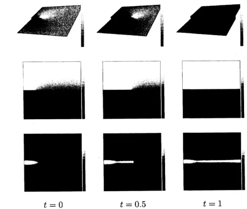
$t=0$ $t=0.5$ $t=1$

We studied that crack evolution phenomena

can

bedeveloped bythe

numer-ical

simulations

of (1) with $g(x, t)$ ([2],[3]). In this _{model, quasi-static}

energy

relaxation that leads the crack evolution is assumed, then,

we

confirm that this

assumption is kept in the numerical simulation.

Set

the initial crack at $t=0$, we make a numerical simulation fixed the

boundary condition

as

$g(x, t)=g(x)$

.

In the following simulations,

we

put

$\epsilon=10^{-3},$ $\alpha_{1}=0,$ $\alpha_{2}=10^{-3},$$\gamma=0.5$ in (1), and set the computational domain

as

$\Omega=(-1,1)\cross(-1,1)$, with $\Gamma_{D}=\{(x_{1}, x_{2})|x_{1}\in(-1,1), x_{2}=\pm 1\}$

.

The

boundary condition for $u$ is given

as

$g(x, t)=5x_{2}(x\in\Gamma_{D}, t\geq 0)$

.

Time

Figure

3:

Temporal evolution of$\mathcal{E}$ (solid line), $\mathcal{E}_{1}$ (dashed line), $\mathcal{E}_{2}$ (dotted line).

The temporal evolution of $u$ (Figure 2) shows the crack evolution, however,

velocity of the crack expansion

becomes

slower by time. From the results of

numerical simulation,

we

calculate the

energy

of system (2). Figure

3

shows

the temporal evolution ofenergy that the elastic energy $\mathcal{E}_{1}$ is decaying, surface

energy$\mathcal{E}_{2}$ is growing, and total energyis decaying slowly

as

the crack growth till

the material is fractured $(t\sim 1)$. We confirm thatthese numerical results follow

our

model and describe the crack evolution phenomena, The physical

character-istics of the material

can

be estimated by calculating the stress intensity factor

from these numerical results.

References

[1] G. A. Francfort and J.-J. Marigo, Revisiting brittle fracture

as an

energy

minimization problem. J. Mech. Phys. Solids, 46 $(1998),1319-1342$

.

[2] T. Takaishi and M. Kimura, Phase field model for mode III crack growth,

[3] Takeshi Takaishi, Mode-III kiretsushinten no phase field model to

sono