The Transient Behavior of the PH/M/S/K Queue

Journal of the Operations Research Society of Japan

Vol. 28, No. 1, March 1985

THE TRANSIENT BEHAVIOR OF THE PH/M/S/K QUEUE

Fumiaki Machihara

Musashino Electrical Communication Laboratory, N. T. T.

(Received April 7, 1983. Final June 5, 1984)

Abstract We analyze the transient behavior of the PH/MI S/K queue. Emphasis is placed on the overflow process, busy period distribution, idle period distribution, accepted arrival process, departure process and the transition probabilities of the system states. All results are represented by the addition and multiplication of the matrices whose dimensions are at most equal to the number of phases for the inter-arrival time distribution.

1. Introduction

The GI/M/S/K queue with S servers and K-S waiting positions is one of the basic models in Telephony, because many queueing syst('ms in telephone network have non-Poisson arrivals such as overflows. In this paper, the PH/M/S/K queue is considered and inter-overflow tlme density function, all-busy period density function, idle period density function, inter-accepted-arrival time density function, inter-departure time density function, transition probabili-ties of the system states and so on are analyzed using Laplace transforms. All the formulae are given by simple recurrences and have a great adVanL!ge in numerical computation. Moreover, these formulae have much applicability. For example, we can obtain the moments o.E overflow traffic by the Laplace transform of the inter-overflow time den.3ity function, using the theory of GI/M/co queue. (5)(15) The Laplace transforms of the all-busy period density function and the inter-departure time density function are important in the analyses of priority queues and tandem queues, respectively. The unsolved model PH[Xj+PH/M/S/K queue with mixed group PH-renewal arrivals and simple PH-renewal arrivals become possible to bl~ analyzed by applying the Laplace transforms of the transition probabilities of the system states to the theory

(6)(9)(11)

of piecewise Markov process. Another paper will discuss these applications in detail.

2 Fumiaki Machihara

There are a number of papers in which the transient behavior of the Gl/M/S/K queue have been studied. In regard to the overflow

process,~inlar-. (4) b (12) d 1 . h h GI/M/l/K d

Dlsney and Matsumoto-Watana e ea t Wlt t e queue an

H2/M/S/K queue, respectively. We can extend their results and also simplify their computation methods.

. f / / / h b d· d b R· h (14)

The busy perlod or the Gl M S K queue ave een stu le y aJu-B at , but their computation algorithm is complicated except for Poisson arrival case. Our results simplify their algorithm and the moments of the busy period can be easily computed.

The accepted arrival process for the loss system Gl/M/S/S queue have been studied by Heffes-Holtzman. (8) They characterize this process as a semi-Markov process. We also characterize the accepted arrival process for the PH/M/S/K queue as a semi-Markov process which depends on the number of

cus-. h d · . k . (13)

tomers ln t e system an derlve a seml-Mar ov matrlX.

Departure processes have been analyzed by Laslett(10) for the GI/M/l/K queue, and have been analyzed by Heffes(7) for the H2/M/S/K queue. In this paper, for the more general model PH/M/S/K queue, the departure process is characterized as a semi-Markov process which depends on the number of cus-tomers in the system and the arrival phase states and a semi-Markov matrix(13) is derived.

The transition probabilities for the system states have been analyzed by Bhat. (1) However, the computational algorithm is complicated. We propose simpler computational algorithm.

2. Model and Notation

We consider the finite queueing system PH/M/S/K. Suppose that the inter-arrivals of customers are mutually independent and identically distributed with a phase type distribution whose density function is f(t) and the service times of customers are independent and exponentially distributed with the mean

lJ-1•

Let us assume that the total number of phases of f(t) is m and assign a number to each phase. Let A

=

{1,2, ..• , m} denote the space of the numbered phases and consider a stochastic process {w(t) E A; t ~ O}. Additionally, let us consider another stochastic process {y(t); t ~ O} where Y(t) signifies the number of customers in the system. It is clear that the bivariate stochastic process {y(t), W(t); t ~ 0 is Markovian.

Transient Behavior of PH/M/S/K Queue

3. First Passage Time Density Functions and Their Application

3.1. First Passage Time Density Functions

Define the density function of thE first passage times (first entrance times (2» in the bivariate stochastic process {Y(t), W(t); t?:;O,

~Y(t)~K,

l~W(t)~m} as follows:

(1)

(3)

and

(4 )

g: (t;n)dt ~p{Y(x)=n+l for some xr(t, t+dt) , Y(y)~ for all y£[O,t]

~.

--I

Y(O)=n, W(O)=i}, O~n~K-l, l~i~m,

+

gi. (t;K)dt ~ P{an overflow occurs at so~e xr(t, t+dt) for the first time after time

°

I

Y(O):,K, W(O)=i}, l~i~m,

g~/t;n)dt !J,. p{Y(x)=n-l, w(x):,j for some xr(t, t+dt), xr(t, t+dt), Y(y)~n for all yr[O,t], no overflows occur in [O,t]

I

Y(O)=n, W(O)=i}, l~n~ K, l~i, j~m,

+

g-. .(t;n)dt

!:,

p{Y(x)=n-l, W(x):j for some xr(t, t+dt) , y(y)~n for all ~J

yr[O,t]

I

Y(O)=n, W(O)=i}, l~n~K, l~i, j~m.

3

We will introduce the definitions (5)~(10) in order to ana]yze (1)~(4). First, let us define the first passage time density functions for transi-tions of the number of customers in the system.

(5)

(6)

(7)

(8)

t'~ (t;n)at ~ p{Y(x)=n+l for some xr(t, t+dt), Y(y)=n for all yr[O,t]

1..

I

Y(O)=n, W(O)=i}, O~n~K-l, l~i~m.

f~ (t; x)dt ~, P{an overflow oceurs at xr(t, t+dt) for the first time

~-after time 0, Y(y)=K for all yr [0, t]

I

Y(O)=K, W(O)=i},

l~i~m.

f~ .(t;n)dt ~ p{Y(x)=n-l, W(x)':j for some xr(t, t+dt) , Y(y)=n for all

~J

-ydO,t]

I

Y(O)=n, W(O)=i}, l~n:;;K-l, l~i, j:;;m.

f-.

.(t;K)dt ~ p{Y(X)=K-l, W(x),:j for some xr(t, t+dt), Y(y)=K for all

~J

--yr[o,t], no customers a"rrive in [O,t]

I

Y(O)=K, W(O)=i}, 1:;;i, j~m.

f± .(t;K)dt ~ p{Y(X)=K-l, W(x)"j for some xrCt, t+dt), y(y)=K for all

4 Fumiaki Machilutra

(9) yE[O,t]

I

Y(O)=n, W(O)=i}, l:iii, j~m.

Next, let us consider the following transition probabilities of phase states.

( 10) O:iin:iiK, l:iij:iim.

where tk and tk+O signify the arrival epochs of k-th customers and the instant immediately after this epoch, respectively. Since h+ .(n) (O:iin:iiK) does not

. ]

depend on n, we simply write h+.

_.

instead of h+ .(n) •

] . ]

Let us consider the following matrices:

( 11) G + (t) (g. + (t;n» l:iii:iim _{(mx l matrix) ,}

n ~.

( 12) G -(t) _(g~ .(t;n» l:iii, j:iim (mxm matrix),

n ~]

(13) G±(t)

n (g~ ~] .(t;n» l:iii, j:iim (mxm matrix),

( 14) F+(t) (f~

n ~. (t;n» l:iii:iim (mx l matrix),

(15) F-(t)

n (f~ ~J .(t;n» 1:iii, j:iim (mxm matrix),

(16) F±(t)

n (f~ ~] .(t;n» 1:iii, j:iim (mxm matrix) , and

( 17) H + (h + .) l:iij:iim ( l xm matrix). .]

. (14) ( ) . . k . (13)

Us~ng ~ 17 , we obta~n both the sem~-Mar ov matrlx for the ac-cepted arrival process and that for the departure process. Refer to these in the

Appendix

for more detail. The semi-markov matrix is called the semi-markov kernel in 9inlar. (3)

Now we have the following recurrences, i.e.,

( 18)

( 19) L (F -(d*c + l(dH) + 1'~ 1'F + (d,

1=0 n n- n l:iin:iiK,

where A(t)*B(t) signifies the convolution of A(t) and B(t), and A(t)l* signifies the 1-th convolution of itself.

Proof of (19):

Let us define the following first passage time density matrices

where

+

(g. (t;n;l»

Transient Behllvior of PH/M/S/K Queue 5

+

gi. (t;n;l)dt ~ p{Y(x)=n+1 for some x£(t, t+dt) , Y(y)~n for all y£[O,t], the upward transitions from Y(·)=n-l to Y(')=n occur 1 times in [O,t]

I

Y(O)=n, W(O)=i}, O~n~K,

and

g:. (t;K;l)dt

11

Pian overflow occurs at some x£(t, t+dt) for the first ti.me after time 0, the upward transitions from y(. )=K-1 to Y(')=K occur 1 times in [O,t]

I

Y(O)=n, w(O)=i}.

When we divide the interval [0,

tl

into its subintervals [0,5

1], (51 ,t1], (t

l,S2], (S2,t2], •.. , (t1-1,Sl]' (Sl,t1], (t1,t] where epochs si and t i signify the epoch of the transition from y(. )=n to y(. )=n-l and that from Y(')=n-l to Y(')=n, respectively, the transition probability density matrices of the intervals [0,5

1]' [s.+O,t.](j=l, .•• ] ] + , 1 ) , _ [t.+O, 5'1] ]

Jt

(j=1, ... ,1-1),

[t +O,t] can be represented by F-(t), G l(t), F (t) and F (t), respectively.

1 n n- n n

Since the transition matrices of [5., .s .+0] and [t., t .+0] are rnXrn identity

+ J J J J

matrix and matrix H , respectively, we obtain

(20) G + (t,l) = (F -(t)*G + 1(t)H) + 1* *F + (t).

n n n- n

- + + T T

Since F (t)*G l(t)H (1,1, " ' , 1) «1,1, ..• , 1) (elementwise), the

n

n-right hand of (19) converges. Then we obtain (19). Similarly, we obtain G

;<t)

(22) I (F (t)H + + *G - 1 (t)) *F (t), 1 * -1=0 n n+ n K-1O:n:i:: 1 (n=lf-1, K-2, ••• , 1), and (23) (24) I (F (t)H + + *G-+ 1 (t»' F (t), 1* -1=0 n n+ n K-1t::n~1.

Let i(s) denote the Laplace transform of x(t) and let us consider the following matrices, i.e.,

-+ -+

(25) G (5)

_fl

(g. (s;n» l~i;;;rn

_,

n ~.

(26) [;- (5)

6 (27) (28) (29) and (30) From (31) (32) (33) (34) and (35) (36) -+ G~(s) -+ Fn (s) 'i-Cs) n -+ res) n (19) , we -+ G (5) n Fumiaki Machihara -+ !J, (g-' .(s;n» l~i, j~m

,

~J -+ ~" (f. (s;n» 1;;i~m

,

~. !J,

(r

.(s;n» ~J 1;;;i, j~m

,

-+

=

( r .(s;n» 1;;;i, j;;;m ~J

obtain the following equations.

-+ -- -+ +-- -+ -1 +-+

F (S)+F (s)G 1(s)(1-H F (s)G 1(5» H F (s),

n n n- n n- n

l~n;;;K.

In a similar fashion, from (21)~(24), we obtain the following equations.

;;- (s) n F~(S) , -- -+ +-+ -+ -1 +-+ --F (s)+F (s)(l-H G- l(S)F (s» H G- l(S)F (s), n n n+ n n+ n + -- -+ Since H , Fn(S) and G

n_1(s) are 1xm matrix, mXm matrix and mx1 matrix,

+-- -+ -+

respectively, H F

n(S)Gn_1(s) in (32) is scalar. Hence, Gn(s) can be easily computed by the addition and multiplication of matrices whose dimensions are m at most. Complex procedures such as the computations of matrix inverses

+ - -+ + ± +

are not necessary at all. Since H G

n+1(S)Fn (S) in (34) and H Gn+1(S)Fn (S) in

-- -+

(36) are scalar, the same conclusion follows for G (s) and G-(s), respectively.

n n

-+ -- -+

Our algorithmic procedures to compute G (s), G (s) and G -(s)

n n (12)n

than the known procedures such as Matsumoto-Watanabe and

are much simpler R · aJu-Bh at (14) . In

Transient Behaviorof PH/M/S/K Queue 7

3.2. Inter-Overflow Time Distribution and Overflow Traffic

The Laplace-Stieltjes transform ~(s) of the inter-overflow time distribu-tion can be represented using (17) and (25) as follows:

(37)

Since the overflow-process from the, PH/M/S/K queue is renewal, we can quantify overflow traffic using the theory of the Gr/M/- queue.(15)(6)

Examp 1 e 1. Overfl ows from the Hm/M/S/ K queue

In this example, we assume the inter-arrival time density function f(t)

m m

to be E k.r .exp(-r .t) (k .>0, r .>0, .E k .=1). Next, we assign a number to each j=1 ] ] ] ] ] ~=1 ]

phase as shown in Fig. 1. From the definitions of f~ (sjn),

i-:

.(sjn) and h+.,

~. ~] . ] we obtain (38) (39) and (40) where -+ f . (sjn) ~. + h . = k]., . ] r. ~

(

".

\.I

=

min (n, S) . \.I. n

(i=j)

(ifj) ,

Therefore, from (31) and (32), we obtai.n

(41 ) g. (SjO) -+ ~. g~ (sjn) ~. (42) and then (43) where (43) r. ~ s+r. ~ r. ~ - - - , - + s+ri+\.In / (1 -b = K

8 Fumiaki Machihara

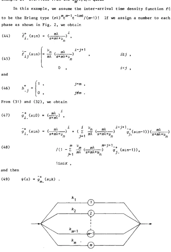
Example 2. Overflows from the Em/M/S/K queue

In this example, we assume the inter-arrival time density function f(t)

to be the Erlang type (wA)mtm-lt-Amt/(m-l)! If we assign a number to each phase as shown in Fig. 2, we obtain

(44) (45) and (46) From (31) (47) (48) and then (49) i -+ mA f. (s;n) = _{(s+mA+lJ )}

,

~. n

--

["n

( mA i-j+l

fi/s;n) = mA _s+mA+lJ ) i"?j

,

n 0 i<j

,

+

-

f~

,

j=m , h .j

_,

Hm and (32) , we obtain -+ g. (s;O) ~. -+ g. (s;n) ~. i i lJ_n A i-j+1_+ mA + (L mA ( m A ) g.(s;n-1)( + A j=1 s+m +lJ_n J. s m +lJ_n m lJ M A m-j+1 /(1 -

L

MA ( m A ) g~ (s;n-l», j=1 s+m _+lJn J. l~n~K , ljI(s) g -+ (s;k) . M. k2 . , . - - - _ \ . 2 r ' -k M ' - -_ _ _ _ _ -\ M } -_ _ _ _ - - - J

Transient Behavior of PH/M/S/K Queue

-0-8--- --

--0--0--Fig. 2 Phase of Erlang Distribution

3.3. Joint distribution of nll-busy period and number of overflows

Since the all-busy period is defined as the first passage time from the epoch at which all servers become busy due to a certain arrival until the epoch at which a server becomes idle as a result of a certain departure, the Laplace-Stieltjes transform, vector B(s), of this can be written as follows:

(50) B(s) - = H Gs(s). +-±

Let T denote the all-busy period and let O(T) denote the number of over-flows in this period. Here, we consider the following joint probability density function.

(51) B(t,j)dt

A

P{t<T~t+dt, O(T)=j}.

Let us define the following first passage time density function with taboo states Y(.) <

s.

g~ (t;n, ~S)dt

A

p{Y(x)=n+l for some x£(t, t+dt) ,

~.

(52) S~Y(y)~n for all Y£[O,t]. no overflows occur in [O,t]

I

Y(o)=n, W(O)=i}, l~i:;;:m .

If we consider the column vector

9

we obtain the following equations 1n a similar fashion to (31) and (32), i.e.,

(53) (54) -+ G (s;YI:::S) n ni1:s+1 . -+ -- -+ +-- -+ -1 +-+ F (s)+F (s)G l(s;Y~S)(I-H F (s)G l(s;Y~s)) H F (s), n n n- n n- n

The Laplace transform B(s,j) of B(t,j), i.e.,

-+ -- +

can be written from the definitions of Gn(s:Y~s), Gn(s), and H as follows:

(55) B(s,j) -

=

H +-+ G (s;Y~S)H +-+ G 1(8;YO:S) .... H GK-l(s;YO:S) +-+

10 Fumiaki Machihara

j?;.O

Specifically, it is clear that

(56)

Therefore, defining

B*(S,Z)

~

fme-st

~

ZjB(t,j)dt,

o

j=O

we obtain from (55) and (56)

(58)

+_+ -1 R-S +_+ + ~s __

+z(1-zH G (s;Y>..s» (IT H G

S+ .(s;Y~S»H ( IT G K- .(s».

K j=O ] j=O ]

Using (58), we can easily compute the covariance Cov(T,O) of the all-busy period and the number of overflows during this period, i.e.,

Cov(T,O) = _{- - - - - B}

a a

-*

_{(s z)}

I

as az ' z=1

s=O

(59)

where BT(s) is a transposed vector of B(S),

and E(O)

a

-- -- -- B(s) as (from (50», +-+ -1 +-+ +-+ -1

(1-H GK(O;Y~S» [1+H GK(0;Y~S)(1-H GK(O;Y~S» ]

R-S R-S

+-+ +

-.( IT H G

_s

+ .(O;Y~S»H ( IT G K_;(O».

j=O ] j = O

-4. Transition Probability

In this section, we consider the transition prnhahility

Transient Behavior of PH/M/S/K Queue 11

Let us introduce

p .. (t;k,l ;n) f::, p{Y(t)=]', W(t)=l, the upward transitions from Y( - )=j-1

]J =

(61)

to Y(-)=j occur n times in [O,t)

I

Y(O)=j, W(O)=k}, and

(62) q .. (t;k,l) ~ p{Y(u)=j for all UE[O,t), w(t)=lIY(O)=j, W(O)=k}_

]J

From (60) and (61),

(63) p .. (t;k,l)

]J _{n=O ] ]} I p .. (t;k,l ;n)_

Let P . . (t;n) and Q .. (t) denote the matrices which have the elements

] ] ]J

Pj/t;k,l;n)(l;;;k, l;;;m) and q j / t ; k , l ) (l;;;k, Hm), respectively, i.e_,

(64) and (65) (p .. (t ;k,l ;n» ]J Q .. (t) = (q .. (t;k,l» ]J JJ

(i) In the case of n

=

0

Considering the number of downward transitions from Y(-)=j+1 to Y(-)=j, we obtain

(66)

'"

L (F + .(dH *G-:++ +

"*

1 (d)"' *Q .. (t)

i = O ] ] JJ

and

(ii) In the case of n ~ 1 From (61), we obtain

(68) (zero matrix),

and

(69) Pj/t;n) = (Gj(t)*G j-1 (t)H) + + + n* *l'j/t;O) ,

Therefore, it follows from (63), (66), (68) and (69) that

(70) and (71) P .. (t) = L (G . ± (t) *G. + (t)8) + n* :, P .. (t ; 0) , ] ] n=o] )-1 .7.7 O;'i;j<K , l;;;j;;;K, n~l _ l$j$ K _

12 Fumiaki Machihara

(72)

+-+ -+

I t should be noted that H G

1

(s)F 0 (s) is scalar.

Taking the Laplace transform of both sides of (71), we obtain

(73) P . . - (s;O)+G .(s)G. -± -+ 1 (s)(I-H +-± G .(s)G. l(s» -+ -1 HP .. (s;O)

+-]J ]

r

]

r

]]

l~j$K ,

where from (66)

(74)

+-+ -+ + - + - +

I t should be noted that H G -: (s)G . 1 (s) and H G -. 1 (s)F . (s) are scalar.

]

r

] + ]

We can easily obtain

O ..

(s) as follows:

]J (75) _Qj/s) Il_j F~(S), ] l$j$K , °KK(s) 1 -+ (76) - - F~(S) • ilK

We can also obtain 000(s) in a similar fashion to 0jj(s) (l$j$K).

(77)

Next, let us consider P . . (t) which is defined as ~]

l$k, l~m, i - f j .

Since P . . (t) is represented as the convolution of the first passage time ~]

from Y(·)=i to Y(·)=j and P .. (t), the Laplace transform

P . .

(s) of pi].(t) can

]] ~] ~ be obtained as follows: (78) P . . (s) ~] -( -+ +-+ + Gi(S)H G_i+ 1 / s)H - + -+ G-:(s)G-: 1 (s) ~ 1 --+ +-G. 1 (s)H P . . (s) , ] - ]J i<j , i>j •

In this way, we have obtained the Laplace transform

P . .

(s;k,l) of the transi-~]

tion of the transition probability P . . (t;k,l) for each i, j, k, 1. ~]

5. Conclusion

We have analyzed the following types of transient behavior of the PH/M/S/K queue. All results are represented by the addition and multiplica-tion of the matrices whose dimensions are at most equal to the total number of

Transient Behavior of PH/M/S/K Queue 13

phases for the inter-arrival time density function. (i) Overflow Process

We have shown that overflows form a rene°.,a1 process and have derived the Lap1ace transform of the inter-overflow time density function.

(ii) Busy Period and Idle Period

We have derived the Lap1ace transform of the busy (idle) period density function.

(iii) Busy Period and Number of Overflo"Is

We have derived the joint distribution of the busy period and the number of overflows during this period.

(iv) Accepted Arrival Process

We have characterized this process as a semi-Markov process and have derived a semi-Markov matrix.

(v) Departure Process

We have characterized this process as a semi-Markov process and have derived a semi-Markov matrix.

(vi) Transient Behavior of the Number of Customers in the System

We have derived the transition probability for the bivariate stochastic process {Y(t), w(t)} where y(t) and w(t) signify the number of customers in the system and the arrival phase state at time t, respectively.

Appendix. Accepted Arrival Process and Departure Process for the PH/M/S/K

Queue

We have considered the process of arrivals which are accepted by the PH/M/S/K queue, and have termed this process the Accepted Arrival Process. In the loss system PH/M/S/S queue, this process is called the Carried Arrival Process. (8)

Let {T.;i = 1, 2, ... } denote the sEquence of times at which arrivals ~

are accepted by the PH/M/S/K queue, and let y(t) denote the number of cus-tomers in this system at time t. Since it .;i = 1, 2, ... } is the subset of

~

time s at which customers arr i ve, {y( T .) ; J = 1, 2, ... } forms an embedded ~

Markov chain. We characterize the accepted arrivals as a semi-Markov process which depends on the number of customers in the system, and derive a semi-Markov matrix (gln(t» 1;<;;1, n~K,

where

(A. 1) gl (t)dtl!.-P{Y(T.)=n,t<T.-T. 1<t:+dtjY(T. 1)=l}.

~-14 Fumiaki Machihllra

For l<K, since the next arrival is always accepted and there is a pure death process between accepted arrivals, we obtain

+ + HF 1(t) , n=1+1, (A.2) H+F-(t)*···*F-(t)*F+ (t) 1 n n-1

o

otherwise, l~l<K •

For l=K, since the next arrival need not be accepted and overflows might occur between accepted arrivals, we obtain

(A.3) [ + + + H F~(t)*F K-1 (t) , + + - - + = H F-(t)*F (t)*···· ·*F (t)*F (t) K K-1 n n-1 '

o ,

otherwise. n=K, l~n<K,

Next, we consider the departure process. Let {6.;i

=

1, 2, ... } denote ~

the sequence of times at which customers in the queue depart. Since {y(o.);i ~

=

1, 2, •.• } does not constitute a Markov chain, we then consider the bivariate Markov chain {y(o.),W(O.);i

=

1, 2, ... }.

~ ~

We characterize the departures as a semi-Markov process which depends on the number of customers in the system and the arrival phase state and derive a semi-Markov matrix (q1n(t;j,k» O~l, n<K, l~j, k~m,

where (A.4)

For n<K-1, since there is a pure birth process between departures, we obtain (A.S) [ F;(t) , + ++ ++

+-=

F ( t ) *H F ( t> * ... *H F ( t ) *H F ( t) 1 1+1 n n + 1 '

o

l::>l~K-1, n=1-1~]f-2, O:;>1:;>K-1, 1~n~K-2, n<1-1:il(-2 •

Transient Behavior of PH/M/S/K Queue 15

(q 1 K-

_,

1 (t) ) 1;;; j, K;;;m (A.6)

0~1~K-1 •

Acknowledgement

The author wishes to express his thanks to Dr. O. Hashida, Mr. K. Kodaira, and Mr. K. Kawashima for their guidance and encouragement.

ReferE!nCeS

[1] U. N. Bhat: Some problems in Finite Queue, Lecture Notes in Eco. and Math. Syst., No.98, PP.139-156, Springer, New York, 1974.

[2] K. L. Chung: Markov Chains with Stationary Transition probabilities, Second Ed., Springer, Berlin, 196/.

[3] E. ~inlar: Introduction to Stochastic Processes, Pretice-Hall, New -Jersey, 1975.

[4] E. ~inlar and R. L. Disney: StrealllS of Overflows from a Finite Queue, Oper. Res., 15, PP. 131-138, 1 967.

[51 V. P. Franken: Erlangsche Formeln fur Semi-Markovschen Eingang, Elec. Infor. Kyb., 4, SS. 197-204, 1968.

[6] M. Fujiki and E. Gambe: Teletraff.ic Theory, Maruzen, Tokyo, 1980. (In Japanese)

[7] H. Heffes: On the Output of a GI/jIII/N Queueing System with Interrupted Input, Oper. Res., 24, PP.530-542, 1976.

r8] H. Heffes and J. M. Holtzman: Peakedness of Traffic Carried by a Finite Trunk Group with Renewal Input, B. S. T. J., 52, PP.1617-1642, 1973. [9] A. Kuczura: Piecewise Markov Processes, SIAMJ. Appl. Math., 24,

PP.169-181, 1973.

[10] G. M. Laslett: Characterising the Finit0 Capacity GI/M/l Queue with Renewal Output, Manage. Sci., 22, PP.l06-110, 1975.

[11] F. Machihara: Traffic Characteristics of Loss System with Two Inde-pendent Renewal Inputs, Trans. IEeE Japan, 63-B, PP.l071-1078, 1980.

(In Japanese)

[12] J. Matsumoto and Y. Watanabe: Theoretical Method for the Analysis of Queueing System with Overflow Traffic, Trans. IEeE Japan, 64-B, PP.536-543, 1981. (In Japanese)

16 Fumiaki Mochiharo

[13] V. Nollau: Semi-Markovsche Prozesse, Akademie-Verlag, Berlin, 1980. [14] S. N. Raju and U. N. Bhat: Recursive Relations in the Computation of

the Equilibrium Results of Finite Queues, TIMS Studies in Manage. Sci., Vol.7 (Algorithmic Methods in Probability), PP.247-270, North-Holland, New York, 1971.

[15] L. Takacs: Introduction to the Theory of Queues, Oxford Univ. Press, New York, 1962.

Fumiaki MACHlHARA: Musashino Electrical Communication Laboratory, N.T.T. 3-9-11, Midoricho, Musashino-shi, Tokyo, 180, Japan.